
AI observability: DCGM metrics, inference SLIs, MFU, cardinality and Xid errors
GPU utilization answers one yes-or-no question: was any kernel running on the GPU? It can read 100% while the deeper DCGM counters show the chip doing a fraction of its work. For training, model FLOPs utilization compares the math the model needs with what the GPUs could do.
What this page answers
Why does GPU utilization show 100% when the GPU is not fully used?
Utilization only says whether any program was running on the GPU during the sample. The DCGM counters beside it, such as SM activity and tensor activity, show how much of the chip was actually working. Read it in “100% busy, 33% useful”
What is MFU in training?
Model FLOPs utilization: the FLOPs per second your model needs on paper divided by the most the GPUs could do at top speed. A dense transformer needs about 6 FLOPs per parameter per token, 2 forward and 4 backward. Read it in “Training: model FLOPs utilization”
100% busy, 33% useful
Remember the fine-tuning job from Down the Wire? It runs on one server with 8 H100 GPUs and gets through 54,600 tokens (roughly, pieces of words) per second. The dashboard is a wall of green:
$ nvidia-smi --query-gpu=index,utilization.gpu --format=csv,noheader
0, 100 %
1, 100 %
... all eight
The output on this page is typical of H100 servers running DCGM 4 and Prometheus. The field names are real. The values are made up to illustrate the point.
So how much of those GPUs' number-crunching power is the job really using?
- About 100%
- About a third
- That number can't tell you
Answer.
$ dcgmi dmon -e 203,1001,1002,1004,1005 -c 3
#Entity   GPUTL  GRACT  SMACT  TENSO  DRAMA
ID
GPU 0     100    0.997  0.621  0.382  0.412
GPU 0     100    0.998  0.617  0.377  0.405
GPU 0     100    0.997  0.624  0.385  0.418
“Utilization” (GPUTL) answers one narrow yes-or-no question: was any program running on the GPU? (A program running on a GPU is called a kernel.) The answer was yes, the whole time. The deeper counters next to it, called profiling counters, tell a different story. The GPU's many small processors (streaming multiprocessors, or SMs) had work in them 62% of the time. The tensor cores, the parts that do almost all of training's math, were busy only 38% of the time.
A number taken from the job itself agrees. 54,600 tokens/s × 6 × 8.03 B parameters ÷ (8 × 989 TFLOPS) comes to 33%. That's the share of the GPUs' top speed spent on the model's real math, called model FLOPs utilization. Neither number means the job is broken. 33% is a decent score for fine-tuning. But “100%” was never the answer to the question anyone was actually asking.
Four GPUs, all at “100%”
The two readings at the top of the page disagreed because they answer different questions. Utilization asks a yes-or-no question for each short slice of time. Was the GPU running any kernel at all?
The deeper counters ask how much of the chip was working, and on what. That matters because those SMs work side by side, and one busy SM is enough to make utilization say yes.
Here's what the GPU is actually doing inside, for four different workloads. Each row is one SM and each column is a slice of time. The grid draws 16 rows to stay readable; a real H100 has 132.
A shaded cell means that SM had work, and darker means busier.
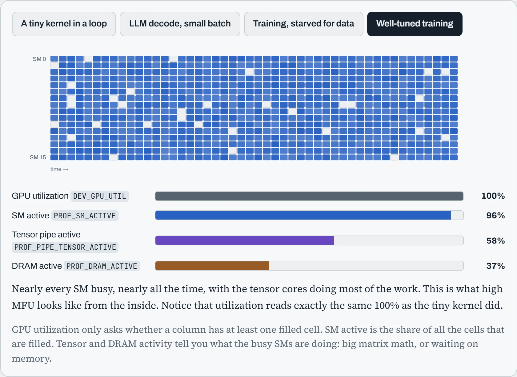
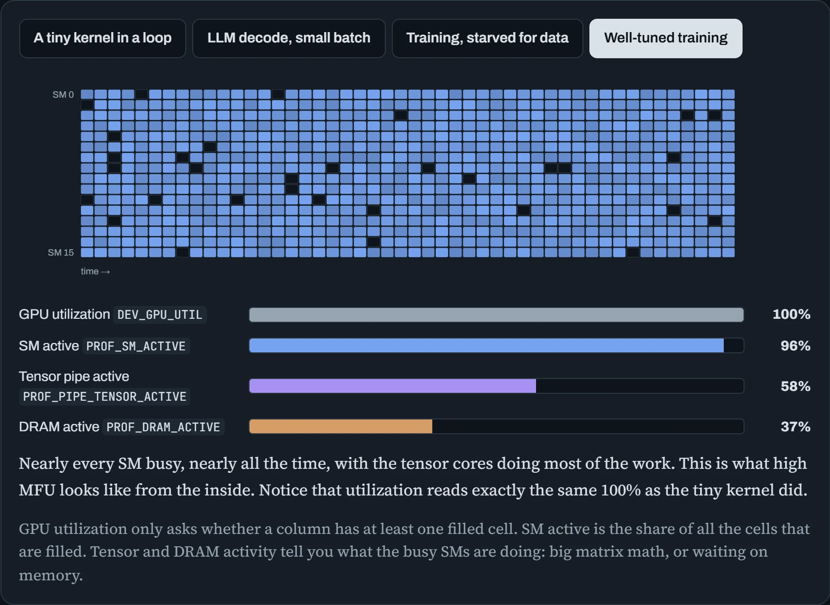
Three of the four workloads read 100% utilization, whether one SM is busy or the whole chip is. The SM active bar is what tells those apart. The last two bars show what kind of busy it is: the tensor cores (the parts built for AI's big multiplications), or DRAM (the GPU's own memory).
Four layers of questions
Good observability (being able to see what your systems are doing) doesn't mean more metrics. It means knowing which question each metric answers. For AI infrastructure there are four, stacked from the machine at the bottom to the users at the top.
The opening example already used two of them. Its 38% tensor-core activity is a layer 2 number, about the chip. Its 33% MFU is a layer 3 number, about the job.
Each band below pairs a layer's question, on the left, with metrics that answer it. The arrow on the right shows the direction you debug in.
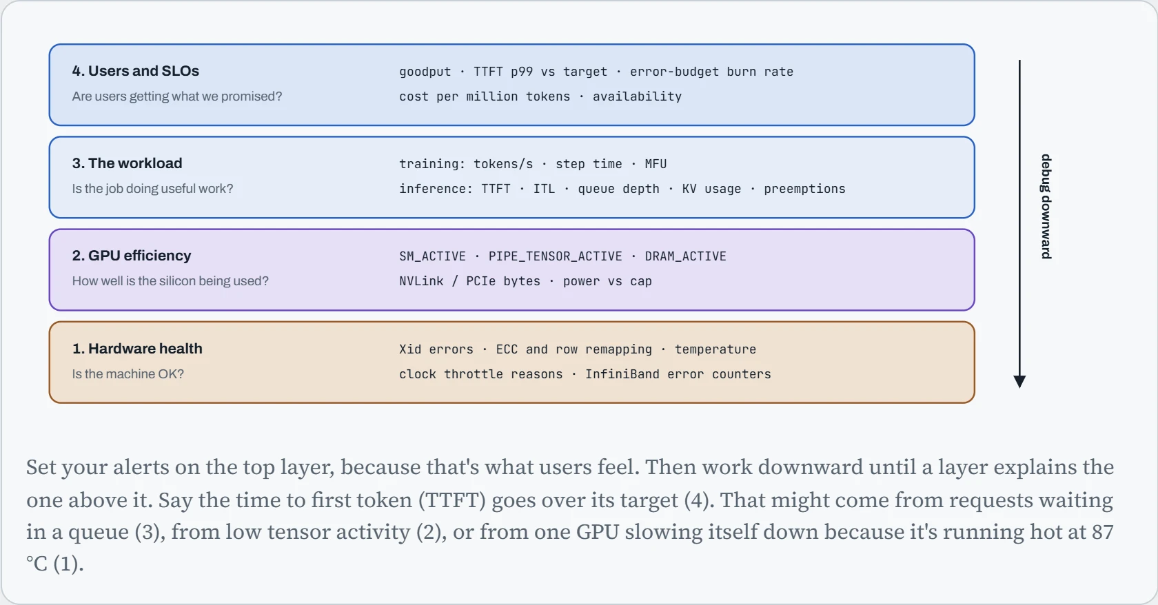
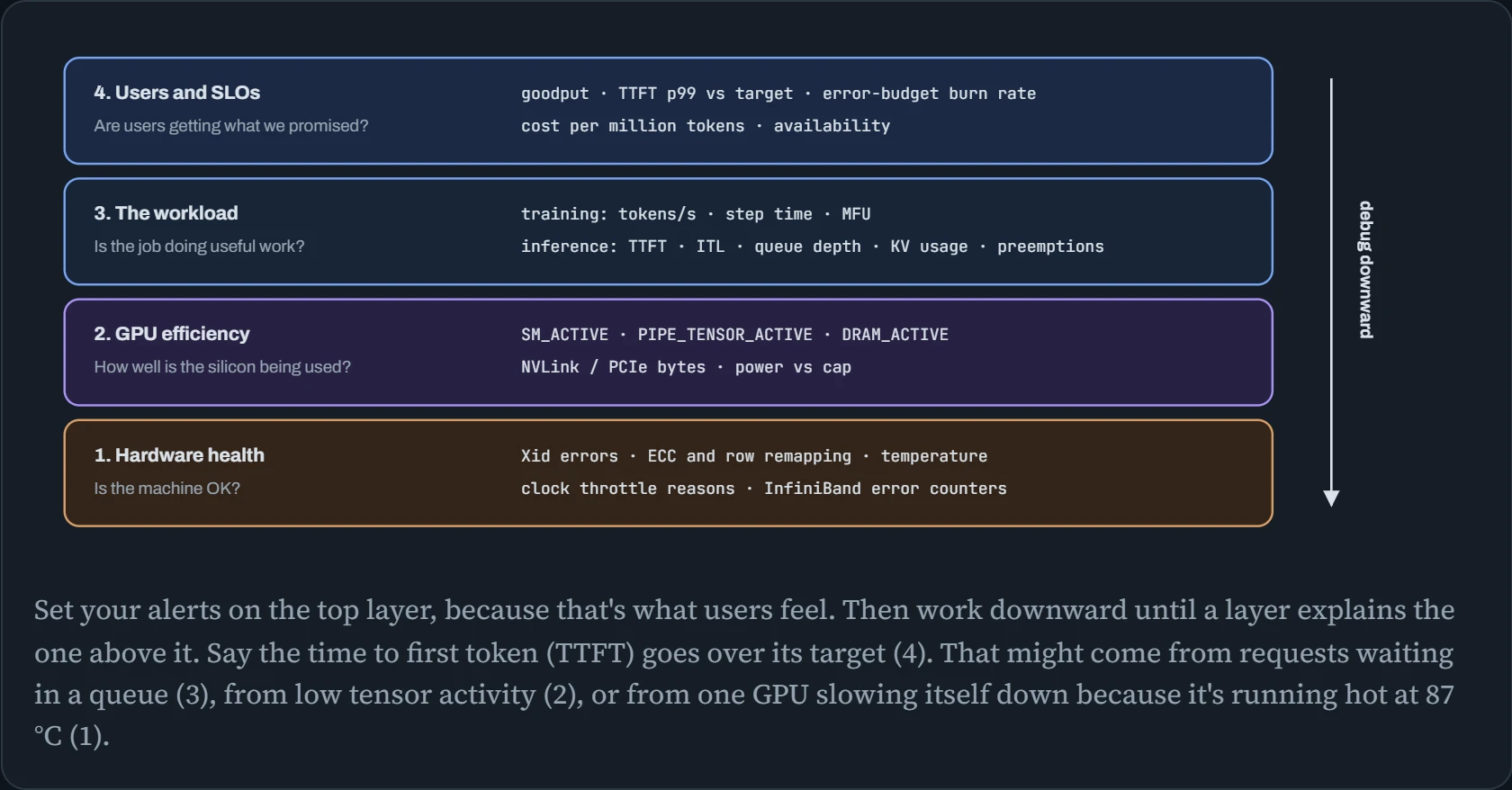
The arrow is the useful part. Start at the bottom and you have a hundred metrics and no question. Start at the top and you have one question, plus a clear next place to look.
From a counter on the GPU to a panel in Grafana
Every number on the dashboard travels the same path. Prometheus, the program that collects and stores them, pulls the numbers in. On a fixed schedule it visits each exporter (a small program that publishes numbers on a web page) and reads its /metrics page. Nothing sends data to Prometheus on its own.
Read the diagram left to right. DCGM, NVIDIA's GPU monitoring tool, reads the GPU's counters. dcgm-exporter then publishes them as a plain-text web page on port 9400. That is all an exporter does: publish numbers on a page like this.
In Kubernetes, the exporter also tags each GPU with the name of the app (the pod) using it. node_exporter publishes the machine's own numbers, like CPU and memory, and vLLM and the trainer publish theirs the same way.
Each visit Prometheus makes is called a scrape, so the arrows point from Prometheus out to the pages it reads. Prometheus stores what it collects. Grafana asks it for numbers to draw panels, and Alertmanager sends alerts on to a pager or chat.
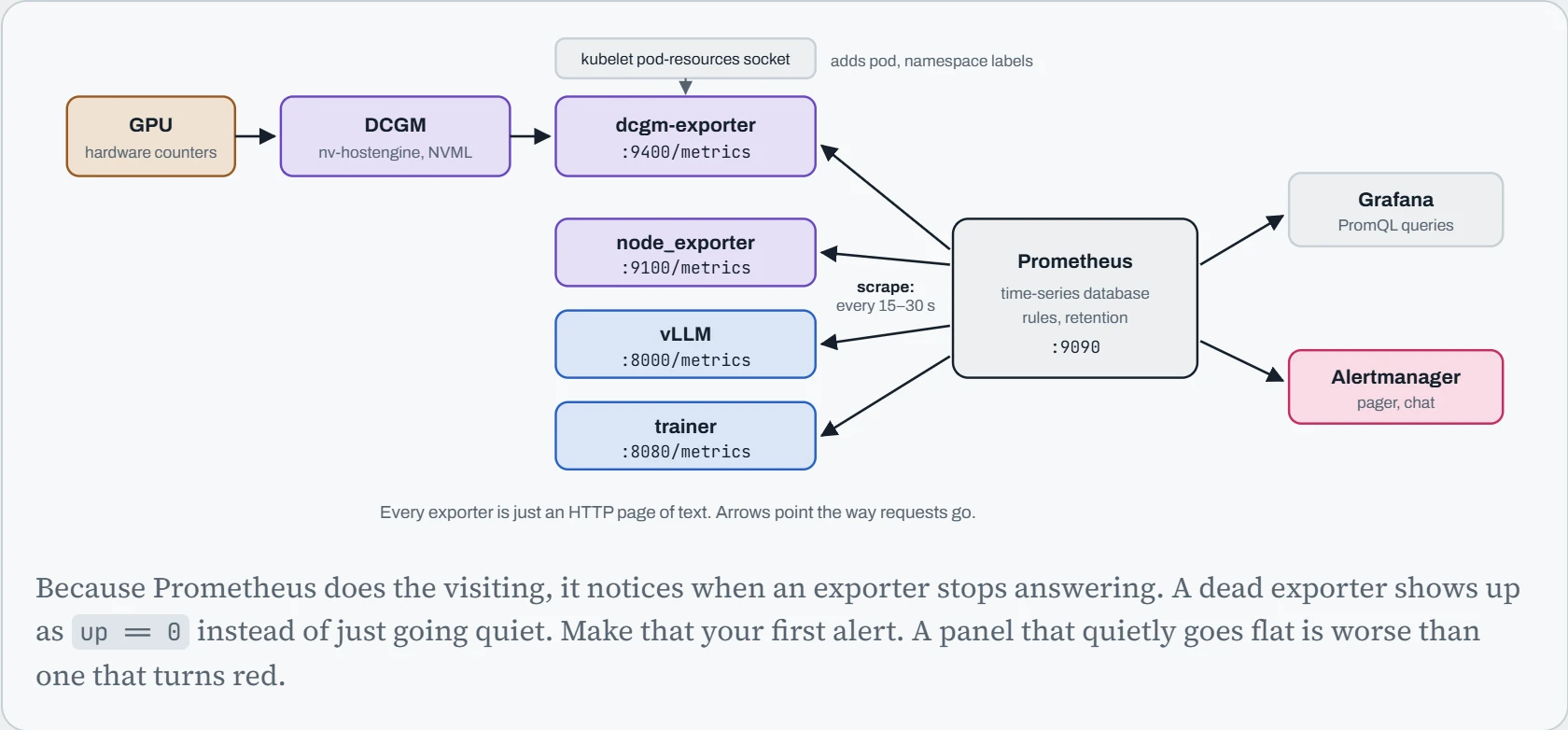
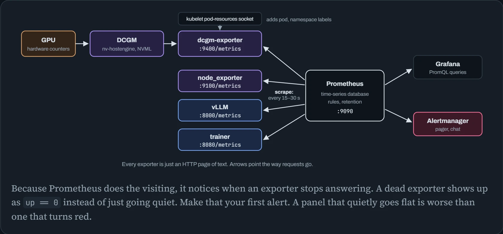
Here's that path done by hand. Start the exporter, fetch its page with curl the same way Prometheus would, then tell Prometheus where to find it. Notice GPU 0 shows the opening example's numbers again: 100 next to 0.621 and 0.382.
# the exporter on a plain GPU host; profiling counters need SYS_ADMIN
$ docker run -d --gpus all --cap-add SYS_ADMIN -p 9400:9400 nvcr.io/nvidia/k8s/dcgm-exporter:$TAG
$ curl -s localhost:9400/metrics | grep -E '^DCGM_FI_(DEV_GPU_UTIL|PROF_SM_ACTIVE|PROF_PIPE_TENSOR_ACTIVE)' | head -3
DCGM_FI_DEV_GPU_UTIL{gpu="0",UUID="GPU-4f1c…",Hostname="gpu-node-1",modelName="NVIDIA H100 80GB HBM3",namespace="team-a",pod="llama-ft-0"} 100
DCGM_FI_PROF_SM_ACTIVE{gpu="0",UUID="GPU-4f1c…",Hostname="gpu-node-1",modelName="NVIDIA H100 80GB HBM3",namespace="team-a",pod="llama-ft-0"} 0.621
DCGM_FI_PROF_PIPE_TENSOR_ACTIVE{gpu="0",UUID="GPU-4f1c…",Hostname="gpu-node-1",modelName="NVIDIA H100 80GB HBM3",namespace="team-a",pod="llama-ft-0"} 0.382
$ cat /etc/prometheus/prometheus.yml
scrape_configs:
  - job_name: dcgm
    scrape_interval: 15s
    static_configs:
      - targets: ['gpu-node-1:9400', 'gpu-node-2:9400']
  - job_name: vllm
    static_configs:
      - targets: ['infer-1:8000', 'infer-2:8000']
In Kubernetes you don't do this by hand. The GPU Operator from Down the Scheduler runs one copy of the exporter on every GPU node (a DaemonSet), and a ServiceMonitor tells Prometheus where they are, instead of a fixed list of targets. The pod labels come from the kubelet, the Kubernetes agent on each node. The exporter asks it, through its pod-resources socket, which pod holds which GPU (each GPU is named by its UUID, a unique ID).
Inference SLIs: measure the users' experience, not the averages
An SLI (service level indicator) is a number that measures what users get from you. For a model server, the top layer is waiting time as users feel it. That's two numbers from Down the Queue: how long until the first token of the answer comes back (time to first token), and the gap between each token after that (inter-token latency). vLLM publishes both as Prometheus histograms. A histogram sorts requests into buckets by time. Each bucket is a running count of the requests that took that long or less:
$ curl -s infer-1:8000/metrics | grep '^vllm:time_to_first_token_seconds_' | sed 's/,model_name="[^"]*"//'
vllm:time_to_first_token_seconds_bucket{le="0.1"} 61844.0
vllm:time_to_first_token_seconds_bucket{le="0.25"} 88214.0
vllm:time_to_first_token_seconds_bucket{le="0.5"} 96930.0
vllm:time_to_first_token_seconds_bucket{le="0.75"} 98602.0
vllm:time_to_first_token_seconds_bucket{le="1.0"} 99211.0
...
vllm:time_to_first_token_seconds_count 100000.0
So 96.9% of this replica's requests got their first token within half a second. Now, the trap. You run two copies of the server (two replicas), and the dashboard needs one p99 for the whole fleet.
A p99 is the wait that 99 out of every 100 requests come in under. The tempting shortcut is to take each replica's p99 and average the two. That treats both copies as equally important, even when one handles half the traffic and the other handles one request in a hundred.
The chart stacks both replicas' waits as bars. Its scale stretches as it goes right, so 50 ms and 10 s fit on one chart. The solid line is the true p99 across every request, and the dashed line is the average of the two p99s.
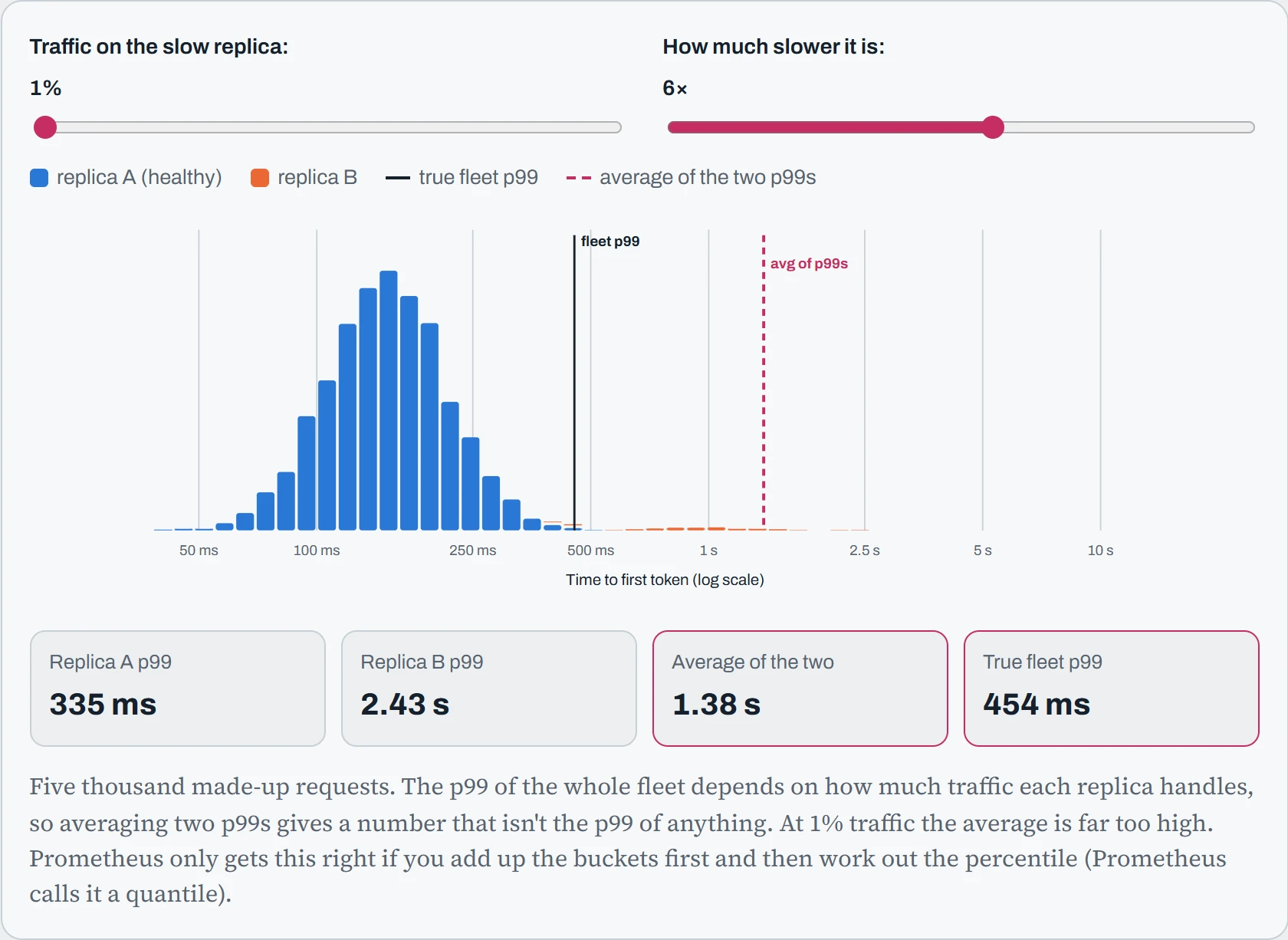
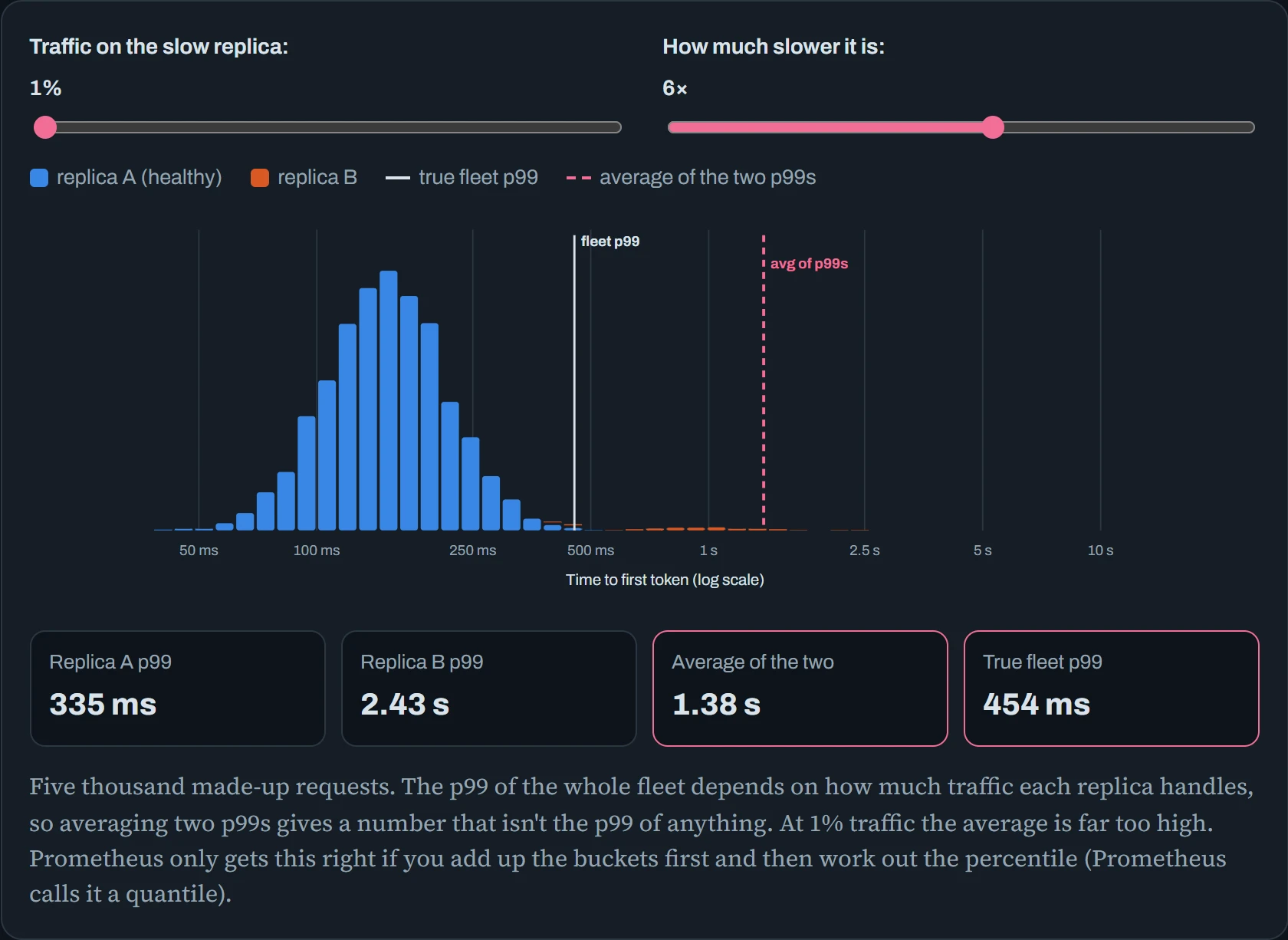
As replica B takes more of the traffic, the dashed line goes from too high to too low. On a real dashboard, nothing would tell you which.
Histograms fix this. Each bucket is just a count of requests, so you can add up the counts from every replica first, then work out the p99 of the total. The first query below does exactly that.
# right: merge every replica's buckets, then take the quantile
histogram_quantile(0.99, sum by (le) (rate(vllm:time_to_first_token_seconds_bucket[5m])))

# wrong: a quantile per replica, then an average of those
avg(histogram_quantile(0.99, rate(vllm:time_to_first_token_seconds_bucket[5m])))

# the SLI itself: the share of requests that met a 500 ms target
sum(rate(vllm:time_to_first_token_seconds_bucket{le="0.5"}[5m]))
  / sum(rate(vllm:time_to_first_token_seconds_count[5m]))
An SLO (service level objective) is the target you aim for, like “99% of requests get a first token in under 500 ms”. Pick targets that sit exactly on a bucket edge. “TTFT under 500 ms” can be counted exactly, because there's a 0.5 s bucket. “Under 400 ms” can only be estimated from the buckets on either side of it.
Next, don't alert on every spike. Alert on how fast you're using up your allowance of slow requests, called the error budget. With a target of 99% under 500 ms, the budget is 1% of requests. The standard rule from Google's SRE workbook sends an urgent alert to whoever is on call when the budget is being used 14.4 times too fast, over both the last hour and the last five minutes. At that speed, a 30-day budget would be gone in about two days:
- alert: TTFTBudgetBurn
  expr: |
    (1 - sum(rate(vllm:time_to_first_token_seconds_bucket{le="0.5"}[1h]))
       / sum(rate(vllm:time_to_first_token_seconds_count[1h]))) > 14.4 * 0.01
    and
    (1 - sum(rate(vllm:time_to_first_token_seconds_bucket{le="0.5"}[5m]))
       / sum(rate(vllm:time_to_first_token_seconds_count[5m]))) > 14.4 * 0.01
  labels: {severity: page}
Training: model FLOPs utilization
For training, the job-level number that matters is MFU. A FLOP is one math step, like an add or a multiply, on floating-point numbers (numbers with a decimal point). MFU takes the FLOPs per second your model needs on paper and divides by the most the GPUs could do at top speed. A dense transformer (a standard model where every parameter is used for every token) needs about 6 FLOPs per parameter per token. That's 2 for the forward pass, which makes a prediction, and 4 for the backward pass, which works out how to improve. On top of that comes an attention term that grows with the length of the text (the sequence length):
MFU = tokens/s × (6N + 12 · layers · d · seq) ÷ (GPUs × peak FLOPS)
Here N is the number of parameters, the model's learned numbers, and the 6N part covers the math done with them. Attention, the step where each token looks back at earlier ones, gets its own term. Its cost grows with the length of the text, so it doesn't fit inside 6N.
Check it against the opening example. 54,600 tokens/s × 6 × 8.03 B parameters, divided by 8 GPUs × 989 TFLOPS (each H100's top speed, 989 trillion operations a second), comes to about 33%.
The calculator starts on that same job. Change the model, the GPU, how many GPUs or the measured speed, and the needle moves across rough bands of MFU.
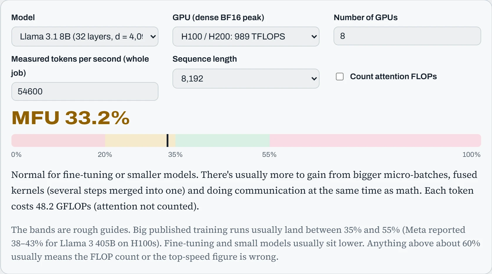
Notice that the calculator never asks for a single DCGM counter. MFU comes from the job's own speed and the model's size, so it can't see how busy the hardware is. That matters as soon as the hardware starts doing extra work.
Predict. You turn on activation checkpointing. To save memory, it throws away some in-between results (activations) and works them out again during the backward pass. Tensor-core activity on the dashboard goes up. What happens to MFU?
Answer. It goes down, or at best stays flat. MFU only counts the FLOPs the model needs on paper, so redoing work earns no credit. The hardware does more math to produce the same tokens per second. There's a separate metric that counts all the math, redone work included, called HFU (hardware FLOPs utilization). That's why MFU, not hardware activity, is the honest number for comparing training setups.
Logs and traces: one request at a time
Metrics describe the whole fleet. When something goes wrong for one user, you need records of individual requests, and there are two kinds. Logs are lines your programs write as they work. Make them structured: one JSON object per line, with the same named fields every time, so a machine can filter them. Then ship them off each server with a collector such as Vector or Fluent Bit into a central store like Loki or OpenSearch, where one query searches every machine at once:
$ tail -1 /var/log/rag-app/app.jsonl | jq .
{
  "ts": "2026-10-25T14:02:11.482Z",
  "level": "info",
  "trace_id": "4bf92f3577b34da6a3ce929d0e0e4736",
  "route": "/ask",
  "model": "chat-8b",
  "prompt_tokens": 1830,
  "output_tokens": 212,
  "ttft_ms": 340,
  "status": 200
}
$ logcli query '{app="rag-app"} | json | ttft_ms > 5000' --since=1h --limit=5
Notice what the log line leaves out: the prompt and the answer. They can contain personal or confidential data, and logs are copied widely and kept for months. A good default is to log sizes, timings and IDs, keep any text in one restricted place with a short retention period, and decide that on purpose rather than by accident. The trace_id field is the bridge to the second kind of record.
Metrics answer “how is the fleet doing?”. They can't answer “why did this request take nine seconds?”, because every request is blended into averages and percentiles. A trace follows one request through every service it touches. Each step becomes a span with a start and an end, and the spans nest: the gateway's span contains the retrieval spans and the LLM engine's span, which contains the queue wait, the prefill and the decode. Read the waterfall below from top to bottom: each bar is one step, placed on a shared clock.
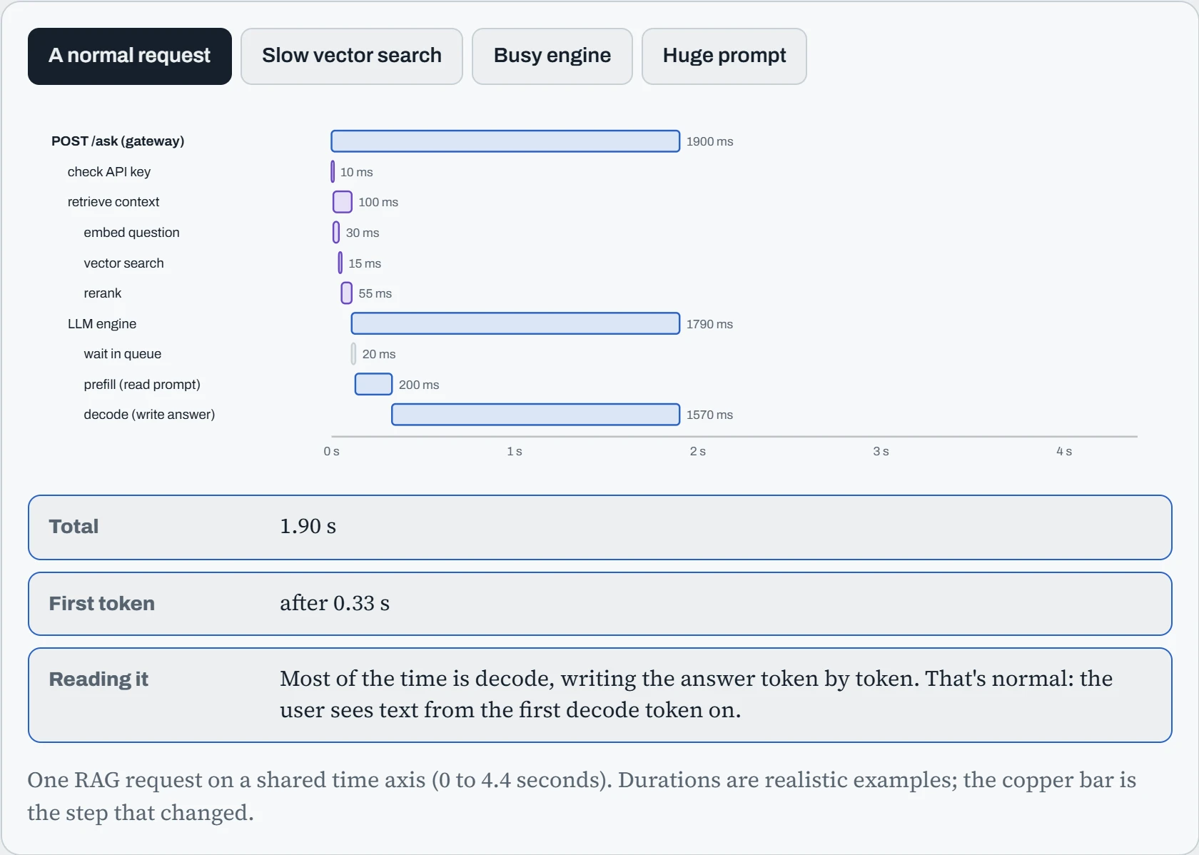
Three very different causes all show up as “slow” on a dashboard, and the trace tells them apart in one glance: retrieval, the engine's queue, or prefill of a huge prompt. Each needs a different fix (an index that fits in memory, more replicas, a context limit). The time to first token is everything before the first decode bar, which links each trace back to the TTFT numbers in the SLI section above.
Continue the lesson
The whole lesson, with its drawings and its questions. The rest of this section and 5 more after it.