
Performance engineering: the roofline model, Nsight profiling, NUMA placement and kernel optimisation
A GPU three times faster can make a job only 1.14 times faster when most of each step is spent elsewhere. Profile from the outside in: Nsight Systems records what the CPU and GPU did in each step. Then the roofline asks whether a kernel is waiting on memory or on math.
What this page answers
How do I find what slows down a training step?
Profile it with Nsight Systems, nsys, which records what the CPU and the GPU did during each step. Labels added to the training code show each part of the step by name, with its time. Read it in “Three times the GPU, 1.14× faster”
What is the roofline model?
Every kernel fetches numbers from GPU memory and does math on them. An H100 fetches about 3.35 TB per second and does about 989 trillion operations per second; whichever runs out first sets the kernel's speed. Read it in “Two ceilings: the roofline”
Three times the GPU, 1.14× faster
A team moves its training job from A100 GPUs to newer H100s. On paper, the H100 does math more than three times as fast, about 989 trillion operations per second against the A100's 312. So each training step should take about a third of the time. Here's what the training log showed instead.
# A100 node
step 200 | 410 ms/step
# H100 node, same code, same batch
step 200 | 359 ms/step      # 1.14x
The timings and profiler output on this page are realistic examples of PyTorch training on 8-GPU servers. The tool commands and flags are real.
Why did three times the math buy only 14%?
- The software isn't tuned for H100 yet
- Most of the step wasn't GPU math
- The model is too small for an H100
Answer. The tool here is a profiler called Nsight Systems (nsys). It records what the CPU and the GPU did during each step, like a stopwatch on every part of the job. The names in the right-hand column are labels added to the training code, so each part shows up by name. Times are in nanoseconds, so 410,216,596 ns is 410 ms.
$ nsys profile -t cuda,nvtx,osrt -o step python train.py --steps 20
$ nsys stats --report nvtx_sum step.nsys-rep
 Time (%)  Total Time (ns)  Instances     Avg (ns)    Range
 --------  ---------------  ---------  -----------    -----------------
     51.6    8,204,331,920         20  410,216,596    :train_step
     19.9    3,166,021,880         20  158,301,094    :dataloader_next
      5.1      812,400,350         20   40,620,017    :log_metrics
Each step took 410 ms, and 158 ms of it was spent just waiting for the next batch of data. A second report lists every GPU job (engineers call them kernels). Adding up their times gives about 80 ms of actual GPU math per step.
The rest went to waiting: for data, for Python to start each small GPU job, for a logging line that made the CPU and GPU stop and wait for each other, and for the network. A faster GPU only shrinks the 80 ms. Real kernels get about 2.8 times faster on an H100, so the step saves about 51 ms. That's Amdahl's law, and it's the first thing to check before buying hardware.
speedup = 1 ÷ ( (1 − f) + f ÷ s )
Here f is the share of the step you're speeding up (0.2) and s is how much faster it gets (2.8). Plug them in and you get 1.14. The H100 was fine. Most of the step simply wasn't GPU work.
Two ceilings: the roofline
Amdahl's law tells you which part of the step to work on. When that part turns out to be one GPU program (a kernel), the same question comes back on a smaller scale: what is this one kernel waiting for?
Every kernel does two jobs. It fetches numbers from the GPU's memory, and it does math on them. Think of a kitchen: ingredients have to come out of the pantry before the cooks can chop anything. An H100 can fetch about 3.35 TB of data per second, and do about 989 trillion math operations per second. Whichever job runs out first decides how fast the kernel goes.
Adding two lists of numbers. For each pair, the GPU fetches 4 bytes, does one addition, and writes 2 bytes back. That's one math operation for every 6 bytes moved. Even fetching at full speed, the math units sit more than 99.9% idle. Faster math won't help at all; only fetching less will.
Multiplying two big tables of numbers (4,096 × 4,096 each). Here every number fetched gets reused 4,096 times. That's about 137 billion operations on only about 100 MB of data. Fetching the data takes about 30 µs, but the math takes at least 139 µs. Now the cooks set the pace.
So the thing that decides which case you're in is how much math a kernel does for each byte it fetches. Engineers call this arithmetic intensity. It's about 0.17 for adding lists and about 1,365 for the big multiply. One line captures both limits:
fastest possible speed = the smaller of ( peak math speed, math per byte × memory speed )
On an H100 the two limits meet at about 295 operations per byte (989 ÷ 3.35). That meeting point is called the ridge. Kernels below it are held back by fetching data, which engineers call memory-bound. Kernels above it are held back by math, which is compute-bound.
The chart below, called a roofline, draws exactly this. Left to right is math per byte, and bottom to top is how fast a kernel actually runs. Each grid line is ten times the one before. The labels use engineering shorthand: FLOPs means math operations, and TFLOPS means trillions of them per second.
The slanted line is the fetching limit and the flat line is the math limit, so together they make a roof. A dot sitting well below the roof is a kernel running slower than the GPU allows.
The blue dots are jobs a language model runs on every training step. There are big and small matrix multiplies (GEMM), FlashAttention (the attention step, written to save memory trips), LayerNorm (rescaling a list of numbers), and GELU (one formula applied to every number). The copper dot is decode, the answer-writing phase of serving from Down the Queue.
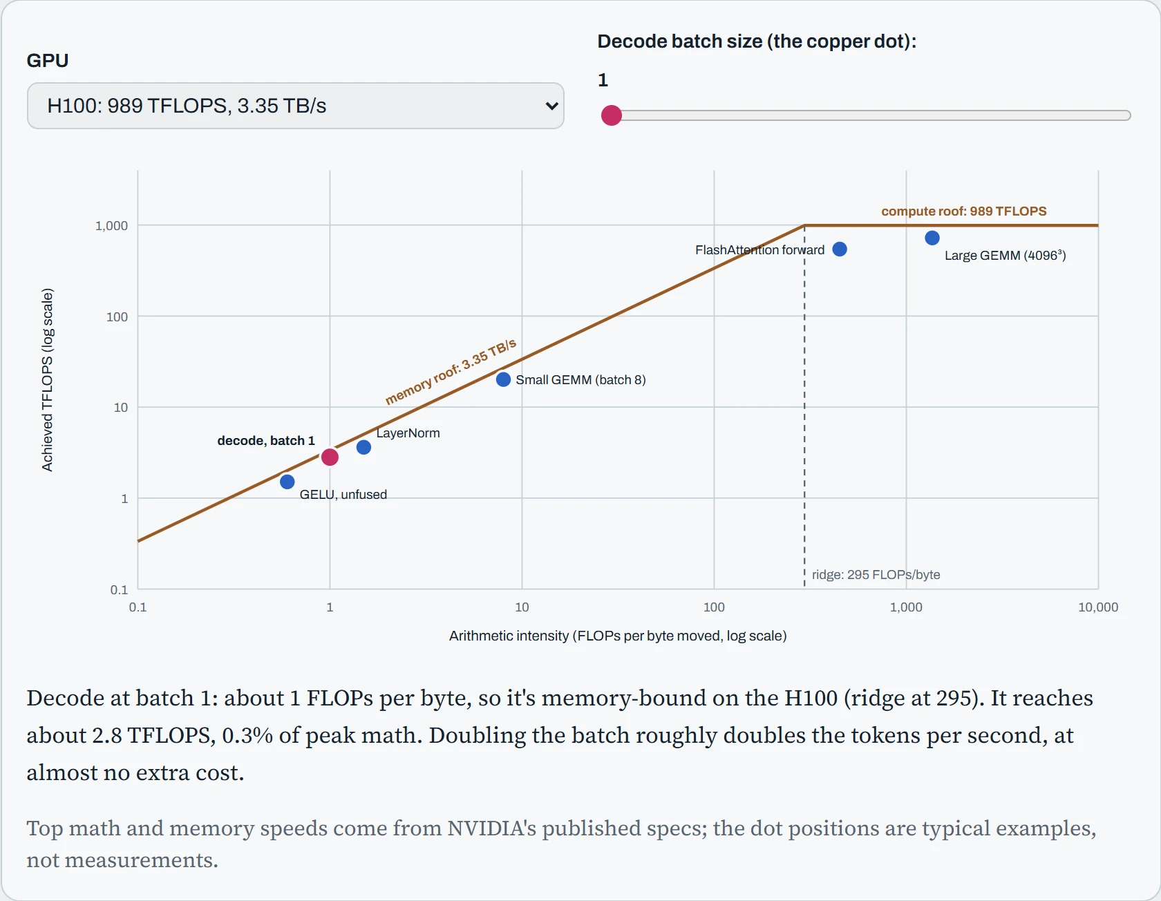
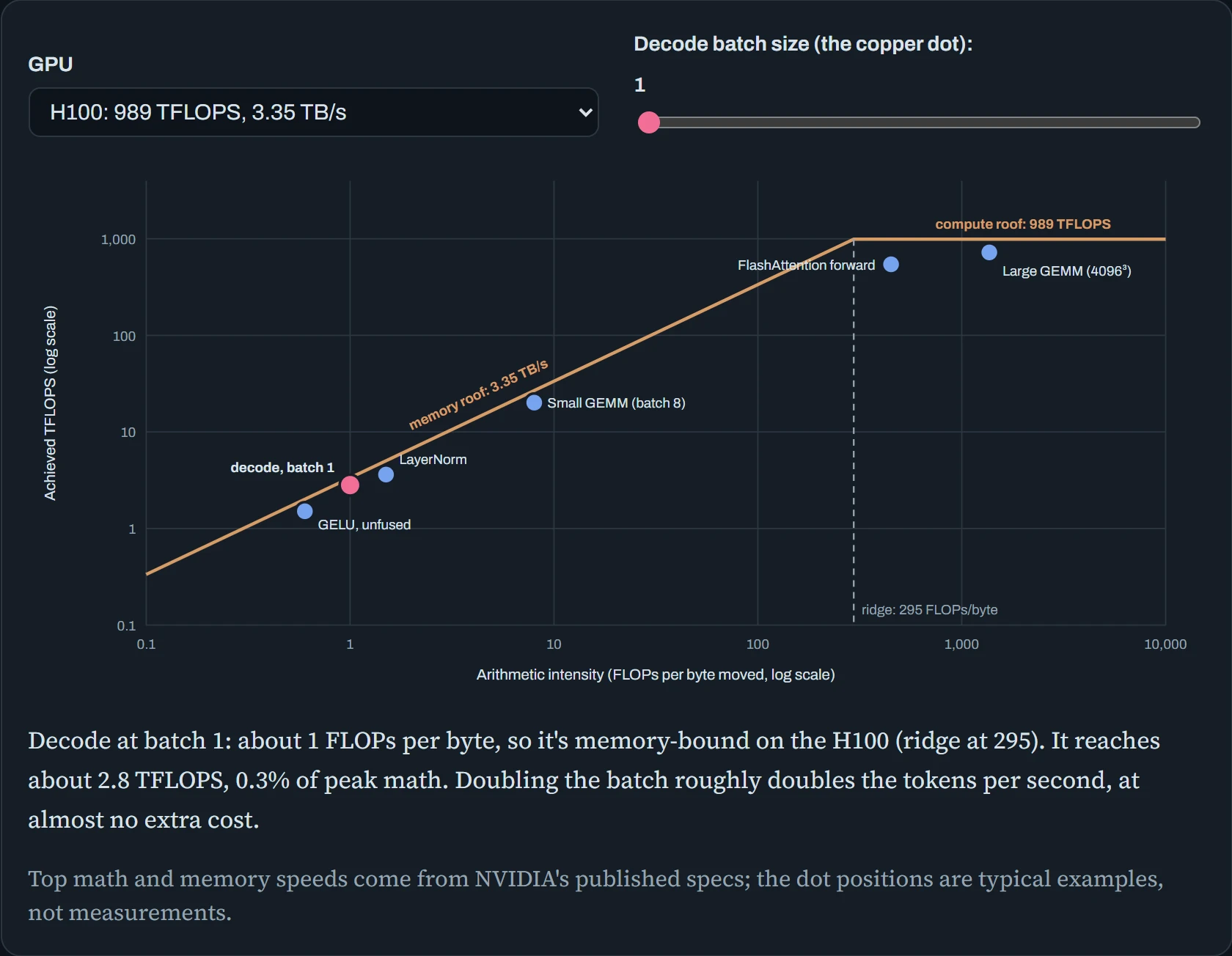
Notice where the dots land. The big matrix multiplies sit close to the flat roof, so they already use most of the GPU. The small, simple operations sit far down the slanted roof, held back by fetching data. Buying more math power does nothing for them, which is part of why the H100 upgrade in the opening helped so little.
Predict. Where does the dot cross the ridge, and what did Down the Queue already tell you about it?
Answer. In a decode step, the GPU fetches the model's weights once and uses them for one new token from each of the B requests in the batch. So it does roughly B FLOPs for every byte it fetches, and the dot crosses the H100's ridge at a batch of about 295. Below that, each extra request costs almost nothing, because it reuses weights the GPU was fetching anyway. That's the 37× throughput jump from Down the Queue, now drawn as a picture. In practice, each request also has its own saved attention data to read (the KV cache), which adds bytes. So the real crossing comes later than the weights alone suggest.
Profile from the outside in
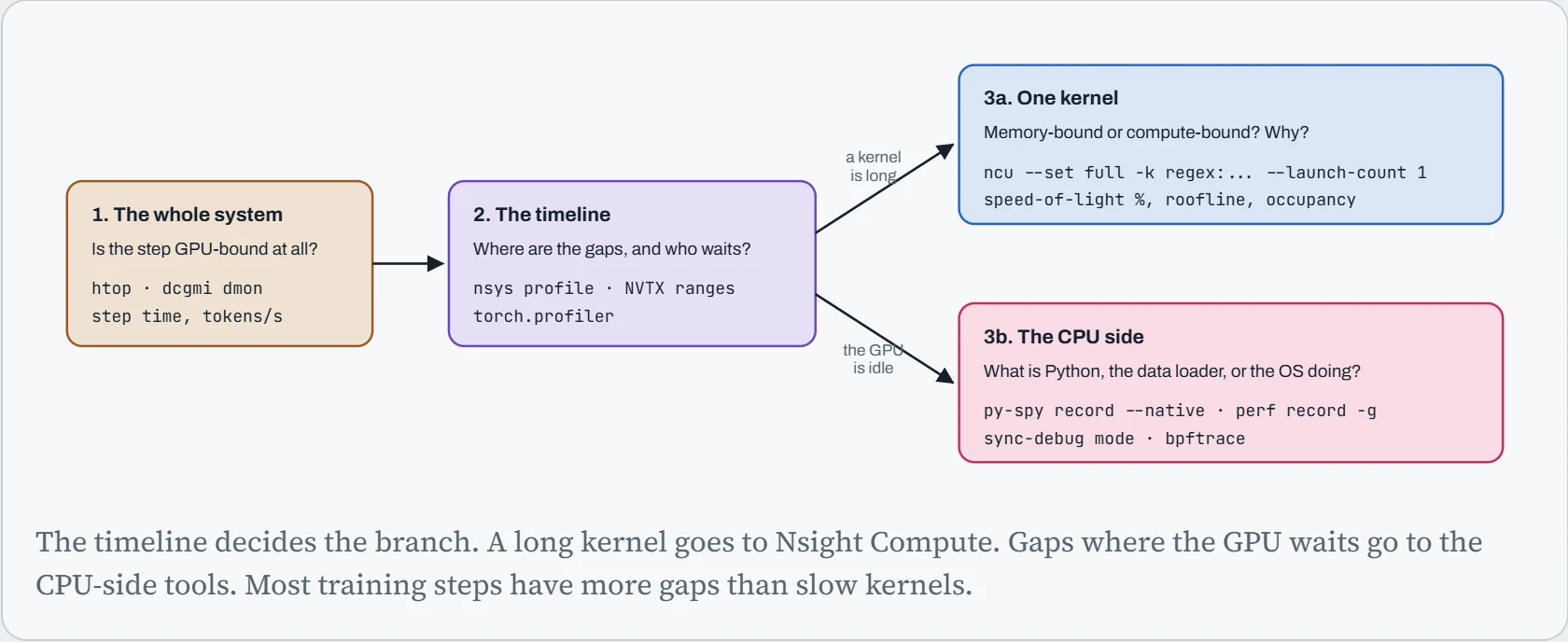
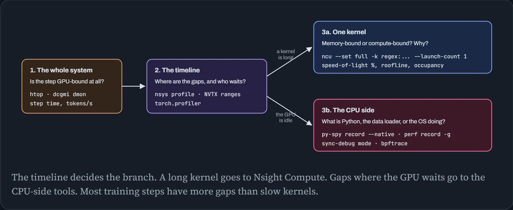
The team in the opening made a classic mistake: they changed something before they knew where the time went. Profiling tools work like zoom levels on a map. You start zoomed out, and zoom in only where the wide view points. Start zoomed in, and you can spend a week speeding up a kernel that was only 3% of the step.
There are three levels. First, the whole machine: is the GPU even the busy part? Second, a timeline: a recording of what the CPU and GPU did, millisecond by millisecond, so you can see the stretches where the GPU sat waiting.
Third, a close-up, which can go two ways. If one GPU kernel is slow, you examine that kernel. If the GPU was waiting on the CPU, you examine the CPU's code instead.
The diagram shows the same path, with the tools for each level. htop and dcgmi dmon show how busy the CPU and GPU are, live. nsys (or PyTorch's built-in profiler) records the timeline. ncu examines one GPU job up close. py-spy and perf show what the CPU was doing. You'll meet each one below.
Step 2, the timeline, is where most answers turn up, so here's how to make one useful. A timeline only makes sense if you label your own code. NVTX “ranges” are those labels. You mark where each part of a step starts and ends, and the parts show up as named bars above the GPU's work. They cost almost nothing to add. These are the labels behind the report in the opening:
import torch.cuda.nvtx as nvtx
it = iter(loader)
for step in range(20):                                   # profile a few steps, not an epoch
    nvtx.range_push("train_step")
    nvtx.range_push("dataloader_next"); batch = next(it);             nvtx.range_pop()
    nvtx.range_push("forward");         loss = model(batch);          nvtx.range_pop()
    nvtx.range_push("backward");        loss.backward();              nvtx.range_pop()
    nvtx.range_push("optimizer");       opt.step(); opt.zero_grad();  nvtx.range_pop()
    nvtx.range_push("log_metrics");     print(loss.item());           nvtx.range_pop()
    nvtx.range_pop()
Now record the timeline, and ask for the GPU jobs that took the most time across all 20 steps:
$ nsys profile -t cuda,nvtx,osrt,cublas,cudnn -o step python train.py --steps 20
$ nsys stats --report cuda_gpu_kern_sum step.nsys-rep | head -5
 Time (%)  Total Time (ns)  Instances   Avg (ns)    Name
 --------  ---------------  ---------  ---------    --------------------------------------------------
     41.2      659,761,920      1,280    515,439    sm80_xmma_gemm_bf16bf16_bf16f32_f32_tn_n_tilesize...
     17.6      281,804,160        640    440,319    flash_fwd_kernel<Flash_fwd_kernel_traits<128, ...
      3.0       47,667,200      8,960      5,320    vectorized_elementwise_kernel<4, GeluFunctor...
The first two lines are big matrix multiplies and attention, the heavy work you'd expect. Now look at the last line. One small operation ran 8,960 times, about 448 times per step, for about 5 µs each. Starting a GPU job from Python takes roughly 10 µs, longer than this one runs. So the CPU spends more time starting these jobs than the GPU spends running them, and the mechanism section shows what that does. A timeline shows this at a glance; a utilization dashboard can't.
Fix the timeline, then buy the hardware
Back to the opening example's 410 ms step. Out of that time, the GPU did useful math for only 80 ms. The other 330 ms it spent waiting, and the waiting came from four different places. Each one looks different in a timeline, and each has its own fix:
Waiting for data (160 ms). The GPU finished one step, and the next batch of training data wasn't ready yet. The helper processes that load and prepare data (DataLoader workers) were too slow or too few. In the timeline, the GPU row goes empty while the dataloader_next label is showing.
Launch gaps (70 ms). Every GPU job has to be started by the CPU. When the jobs are tiny, the GPU finishes each one before the CPU has started the next, so it waits in between. You'll see thin slivers of GPU work with gaps around them, and one CPU core stuck at 100%.
Waiting on the network (60 ms). After each step, the GPUs share their results with each other (chapter 25). If that sharing happens after the math instead of alongside it, everything stops while the network catches up.
Sync stalls (40 ms). Normally the CPU queues GPU work and moves on without waiting. A line like print(loss.item()) needs a real number back, so the CPU stops until the GPU empties its whole queue. Then the GPU sits idle while the CPU fills the queue again. torch.cuda.set_sync_debug_mode("warn") points out every line that does this.
GPU math (80 ms). The only useful part, and the only part a faster GPU speeds up.
The bar below shows the same step, coloured by those five parts, at the scale of the original 410 ms. Before each one, guess which segment will be the biggest afterwards:
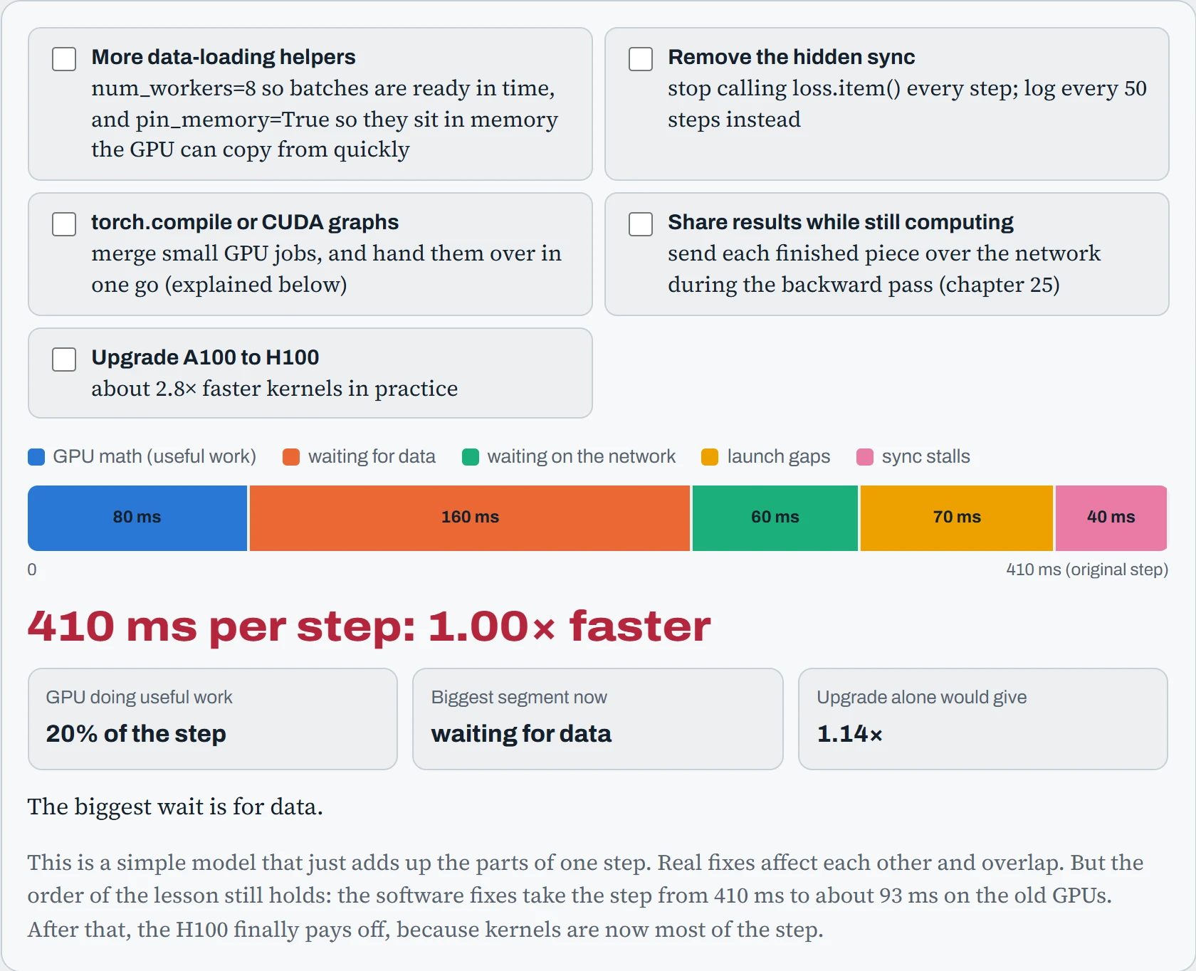
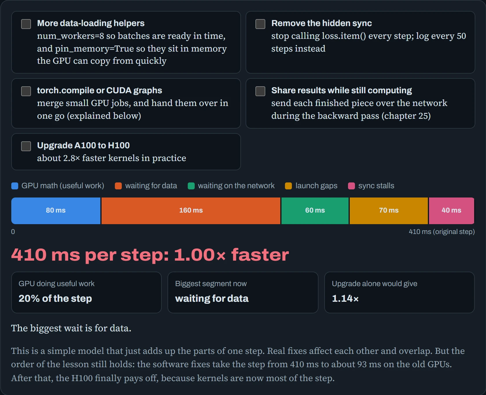
The same H100 gives about 1.14× on the messy step and close to 2× more on the cleaned-up one. The GPU is identical both times. The difference is how much of the step it's responsible for.
Predict. After the four software fixes, GPU math went from 20% of the step to 73%. Use Amdahl's law from the opening: why does the H100 now buy so much more?
Answer. Because f, the part the upgrade speeds up, grew from 0.2 to 0.73. Plug it in: 1 ÷ (0.27 + 0.73 ÷ 2.8) ≈ 1.9×, on top of the 4.4× from the fixes. Together that's the 8.3× the tool shows.
That one sum is the main idea of this page. Hardware only speeds up the part of the time it's responsible for, so first make that part as big as you can.
NUMA: which half of the machine your process lives in
A big GPU server usually has two CPU chips, called sockets. It's really two computers joined by a bridge. Each socket has its own memory sticks plugged in next to it, and four of the eight GPUs are wired to each side (the same layout Down the Wire mapped). Each half, its CPU plus its memory, is called a NUMA node.
Reaching memory on your own side is quick. Reaching memory on the other side means crossing the bridge, which is slower and shared by everyone else crossing it. That's fine for most programs, but a training job moves gigabytes of data to its GPU every few seconds, so the trips add up.
By default, Linux doesn't think about any of this. It runs your threads on whichever cores are free, on either side. And it puts memory on the side of whichever core first writes to it. So a data-loading thread that happens to land on the far socket builds its batches in the far socket's memory, and every batch then crosses the bridge to reach GPU 0.
The diagram shows one server. The pink lines trace every trip the data takes, and any pink line through the bridge in the middle is a slow trip.
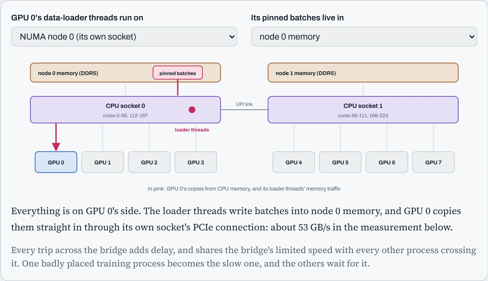
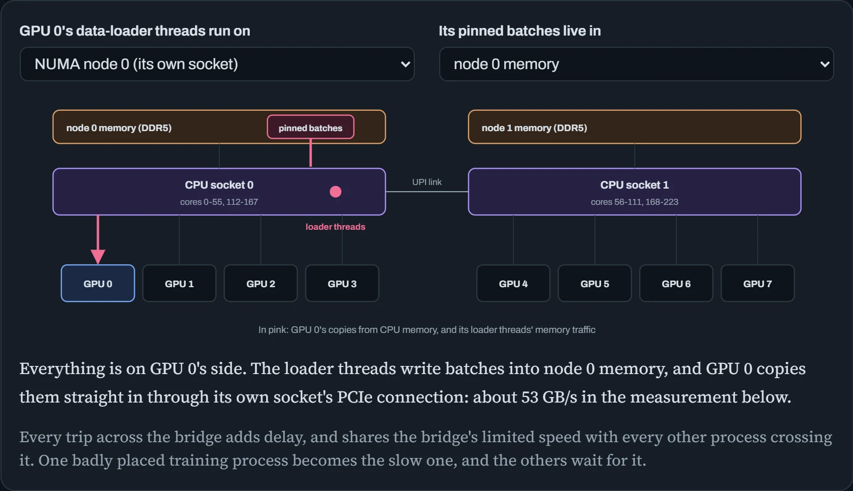
How much does the bridge cost? lscpu shows which cores belong to which side. Then NVIDIA's nvbandwidth tool measures how fast data copies from memory to GPU 0. numactl pins the test to one side or the other, so you can measure the same copy both ways:
$ lscpu | grep NUMA
NUMA node(s):                         2
NUMA node0 CPU(s):                    0-55,112-167
NUMA node1 CPU(s):                    56-111,168-223
$ CUDA_VISIBLE_DEVICES=0 numactl --cpunodebind=0 --membind=0 ./nvbandwidth -t host_to_device_memcpy_ce | tail -1
SUM host_to_device_memcpy_ce 53.24
$ CUDA_VISIBLE_DEVICES=0 numactl --cpunodebind=1 --membind=1 ./nvbandwidth -t host_to_device_memcpy_ce | tail -1
SUM host_to_device_memcpy_ce 39.87                     # GB/s, the same copy across the socket link
About a quarter of the speed disappears when the data lives on the wrong side. In a job with eight GPUs, the one process placed badly becomes the slowest, and the others wait for it every step.
The fix is a few lines: tell Linux to keep each GPU's process on the side that GPU is wired to. The “CPU Affinity” and “NUMA Affinity” columns of nvidia-smi topo -m tell you which side that is. This small script wraps each process in numactl with the right side:
$ cat bind.sh
#!/bin/bash
# run each local rank on the NUMA node closest to its GPU
case $LOCAL_RANK in 0|1|2|3) NODE=0 ;; *) NODE=1 ;; esac
exec numactl --cpunodebind=$NODE --membind=$NODE "$@"
$ torchrun --nproc-per-node=8 --no-python ./bind.sh python train.py
To check that it worked, numastat -p <pid> shows how much of one process's memory sits on each side. For a well-placed process, nearly all of it is on one node.
The rest of the host checklist
These settings matter far less than the timeline fixes, and some do nothing for some workloads. Change one at a time, and measure step time three times before and after: run-to-run noise is often 2–3%.
| Setting | How to check | When it matters |
|---|---|---|
| CPU speed policy (frequency governor) | cpupower frequency-info | grep governor | In powersave mode the CPU runs slower, which slows data loading and kernel launches. Use performance on training machines. |
| tuned profile (a preset for many settings) | tuned-adm active | accelerator-performance or throughput-performance set the governor, the CPU's sleep states (C-states) and other kernel settings in one go. |
| GPU persistence mode | nvidia-smi -q | grep Persistence | Without it, the driver lets go of the GPU when the last program using it exits, then has to set it up again for the next one. That adds seconds to every start. |
| GPU power limit and clocks | nvidia-smi -q -d POWER,CLOCK | One machine with a lower power cap, or a GPU running hot, becomes the slow one everyone waits for (the straggler). Check this before blaming the code. |
| Bigger memory pages (transparent huge pages) | cat /sys/kernel/mm/transparent_hugepage/enabled | Programs with large buffers in CPU memory can run faster. But some workloads get sudden pauses while Linux shuffles memory around to make the big pages (compaction). Measure both ways. |
| Which cores handle network interrupts (IRQ affinity for NICs) | cat /proc/interrupts | grep mlx5 | head | The network card interrupts a CPU core whenever it needs attention. If those interrupts land on the far socket, or on cores busy loading data, they get in the way. This matters for jobs that span several machines. |
Continue the lesson
The whole lesson, with its drawings and its questions. 6 more sections after the ones above.