
The decoder-only transformer block: MLP, residual stream, pre-norm LayerNorm and RMSNorm, RoPE
Attention moves information between tokens but cannot compute anything new, does not know word order, and does not train when stacked deep. A transformer block adds a per-token MLP, a residual stream with normalization, and position information such as RoPE, then stacks the block many times.
What this page answers
Why does a transformer need an MLP after attention?
Attention only takes weighted averages of existing value vectors. The MLP is a per-token non-linear function that turns the gathered information into new features. Read it in “The MLP: where each token does its homework”
What is RoPE?
Rotary position embedding: it encodes position by rotating the query and key vectors by an angle that depends on each token's position, so attention can tell where tokens are. Read it in “Teaching a bag of letters to count”
Attention can move information. It can't think.
You finished the last lesson with a working attention layer. Before you go stacking it into a skyscraper, look hard at what it actually does: every token takes a weighted average of other tokens' value vectors. That's it. It's a superb courier. It is not, by itself, a language model.
Predict first. Using only what you know about attention from the last lesson, list what's missing. What can't a single attention layer do that a language model obviously needs? Aim for three or four things.
Answer. It doesn't know word order Shuffle the tokens and each output just shuffles along. To it, a sentence is a Scrabble rack.
→
Position information Add a “where am I” vector to each token, or rotate q and k by position.
It can only average Outputs are blends of existing values. Nothing genuinely new is computed.
→
An MLP after every attention layer A per-token non-linear function that turns gathered information into new features.
One layer is one hop “it” → “cat” is fine, but “it” → “cat” → “which cat was mentioned earlier” needs a second look.
→
Stack many blocks Each layer can build on what the previous one gathered.
Deep stacks don't train Gradients fade through dozens of layers, and activations drift in scale.
→
Residual connections and normalization A clean gradient highway, plus a volume knob on every layer's input.
Those four fixes, wrapped around attention, are a Transformer block. The rest of this lesson takes them one at a time.
Assemble the block, then try breaking it
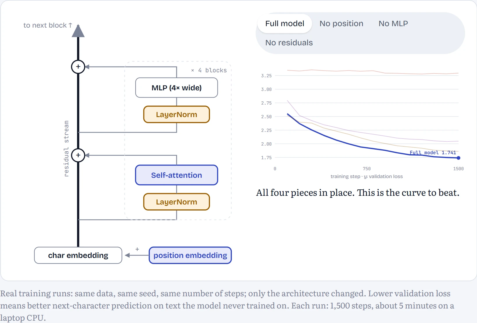
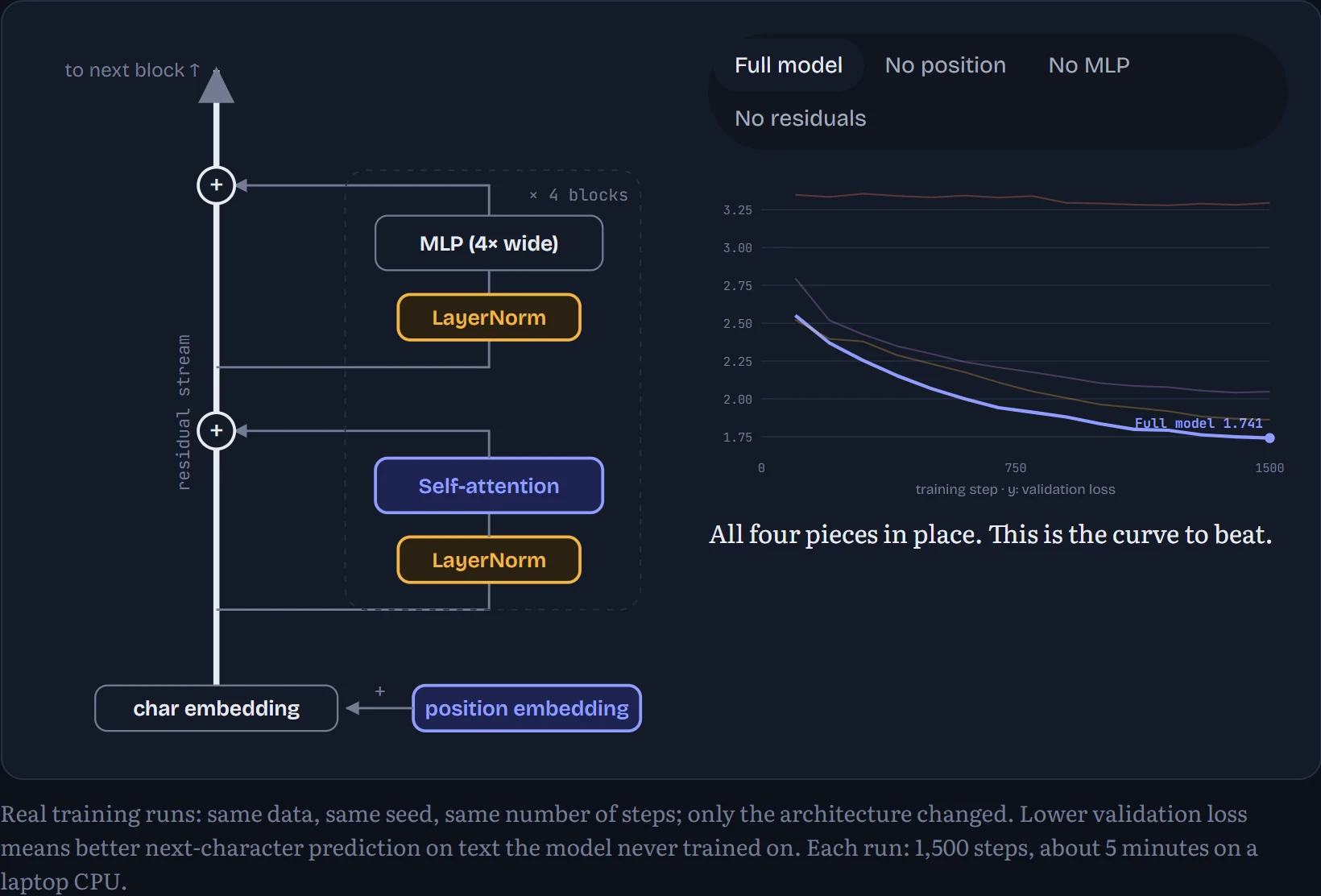
Here's the block our model uses, the same layout as GPT-2 and most models since. Data flows bottom to top. The thick vertical line is the residual stream: each token's running vector. Every sublayer reads a normalized copy of it and adds its result back in.
Claims like “residuals are essential” are cheap, so I didn't just assert them. I trained this exact model four times on the same data with the same seed, removing one piece each time.
How to read it: the diagram on the left is one block, with data flowing upwards. When you remove a piece, it turns faded and dashed in the diagram. The chart on the right is that version's real training run: validation loss over time, where lower means better predictions. The full model's line always stays visible, so you can see exactly how much worse each missing piece made things.
The MLP: where each token does its homework
If attention is a meeting where everyone shares notes, the MLP is everyone going back to their desk and doing the actual work. It runs on each token separately, with the same weights at every position, and nothing crosses between tokens.
Mechanically it's the network from Chapter 5: widen the vector 4×, apply a non-linearity, shrink it back. In our model that's 96 → 384 → 96.
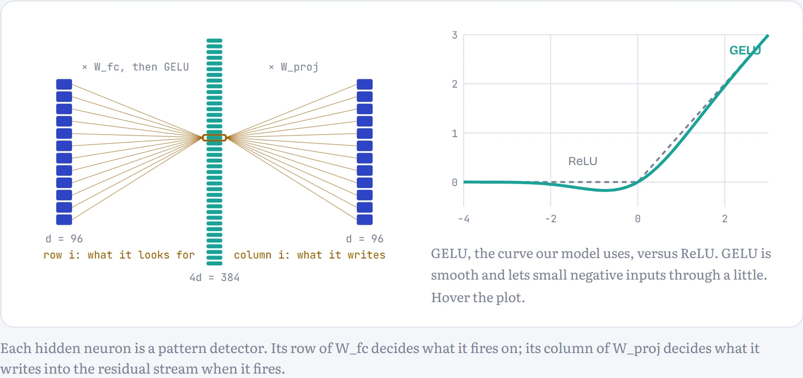
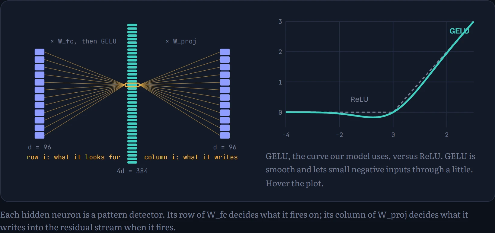
Here's a way to picture it that's mechanically exact. Hidden neuron i takes a dot product between the token's vector and row i of the first matrix. That's a similarity score, just like a query meeting a key. If it's high, GELU lets it through, and the neuron adds column i of the second matrix into the stream. So the MLP is a big bank of “if the stream looks like this, add that” rules, a few hundred of them per layer in our model and tens of thousands in big ones.
That's also where most of the parameters live. Attention has four d × d matrices (4d²). The MLP has two d × 4d matrices (8d²). So about two-thirds of every block is MLP.
OPEN RESEARCH. Interpretability studies find MLP neurons that behave like key–value memories and store many factual associations. It's a productive picture with real evidence behind it, but individual neurons often respond to several unrelated things at once (superposition), so “one neuron, one fact” is too simple.
The residual stream and its volume knob
Picture the residual stream as a shared whiteboard that travels up through the model. Each sublayer reads it, computes something, and adds a note. Nothing is erased; layers can only add. Two good things follow. First, a layer that has nothing useful to say can write almost zero and get out of the way, so adding layers rarely hurts. Second, during backprop the gradient can flow straight down the stream through every “+”, because the derivative of x + f(x) with respect to x always includes a plain 1.
The catch: if every layer keeps adding, the numbers on the whiteboard grow. A sublayer that saw values around 1 during early training might later see values around 50. That's where normalization comes in. LayerNorm is the volume knob that stops each layer from shouting louder than the last.
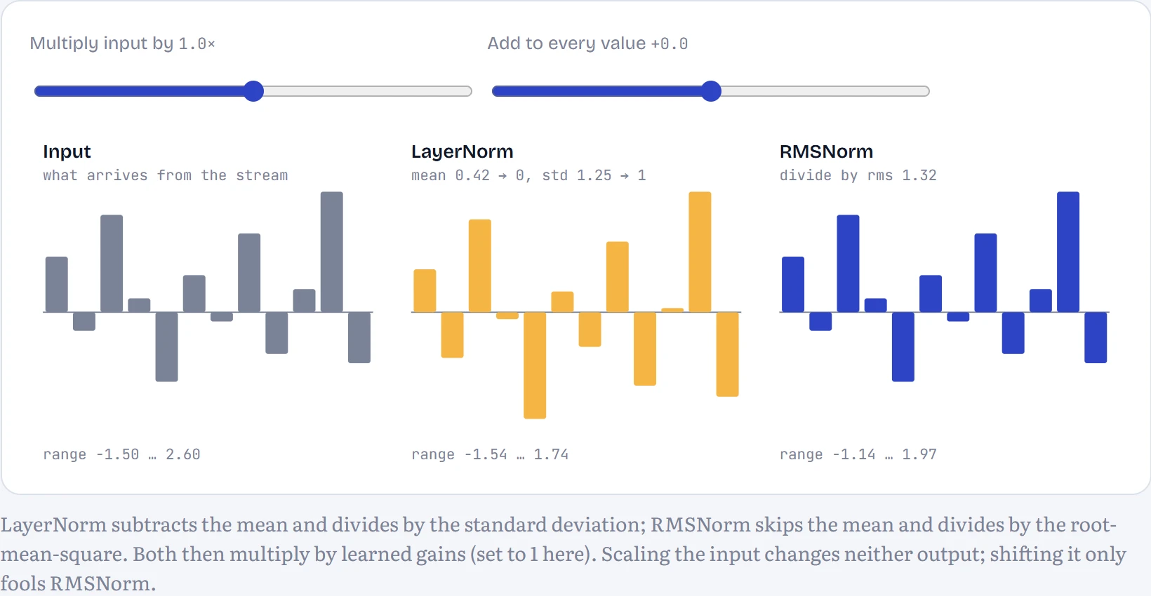
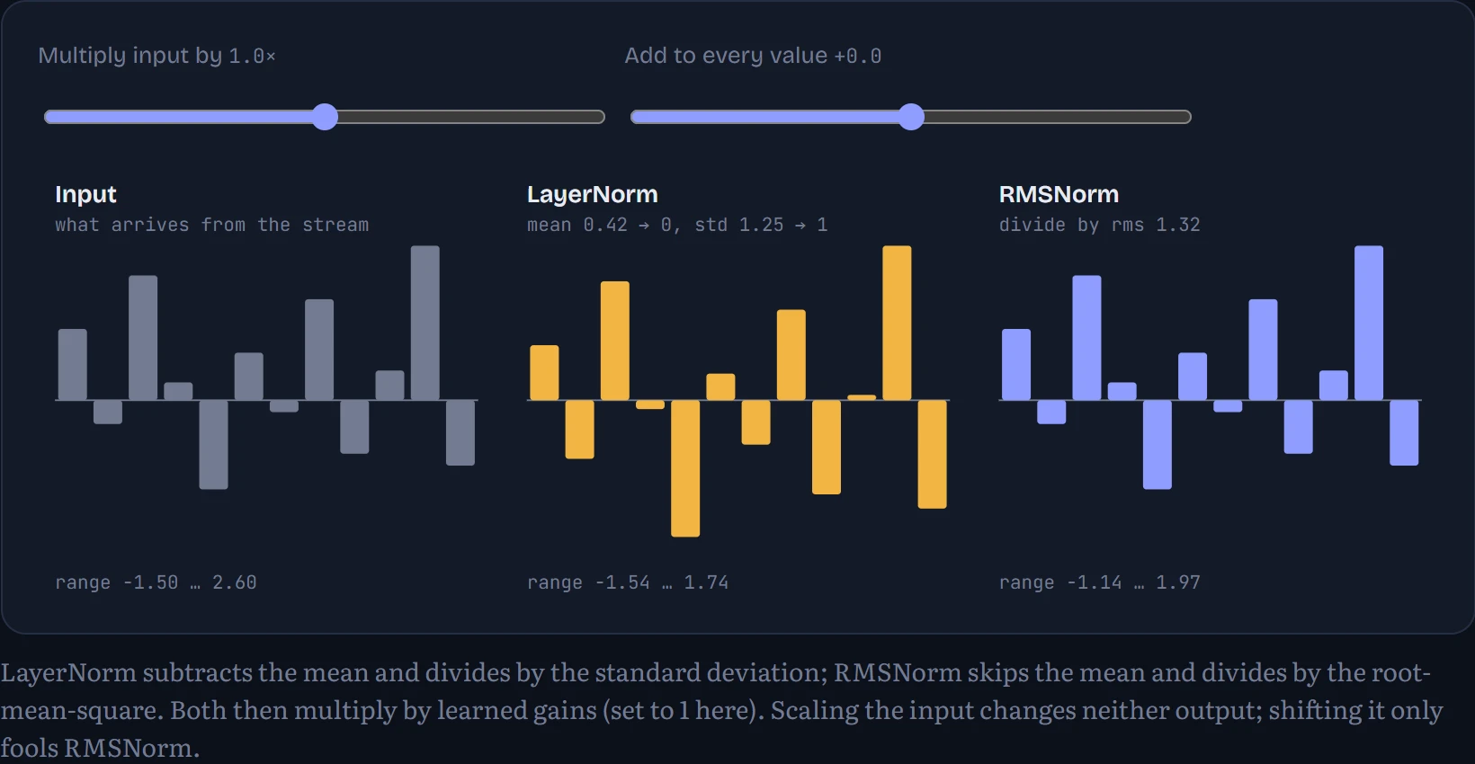
Scale the input up or down and watch what comes out.
How to read it: the grey bars are twelve numbers arriving from the residual stream. The amber bars are the same numbers after LayerNorm, and the blue bars after RMSNorm. Multiply the input and the grey bars grow or shrink wildly, but the amber and blue ones stay exactly the same shape and size: the next layer always receives numbers of a sensible size. Add the same amount to every value and only RMSNorm changes, because it doesn't subtract the average.
Where you put the knob matters
The original 2017 Transformer normalized after adding the residual (post-norm). GPT-2 moved the norm to the start of each branch (pre-norm), which is what our model does. The difference looks cosmetic. It isn't:
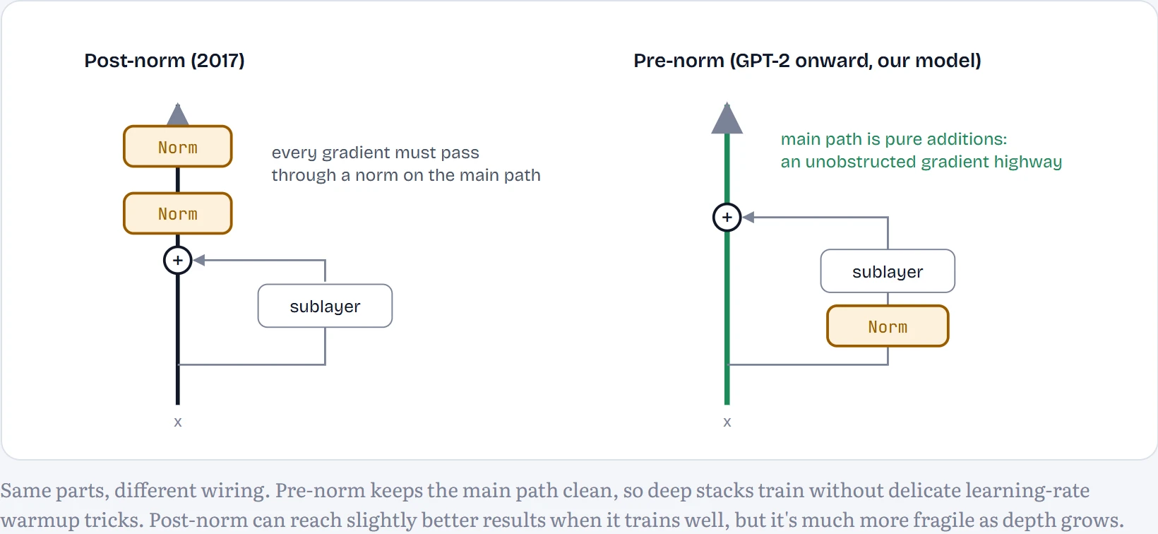
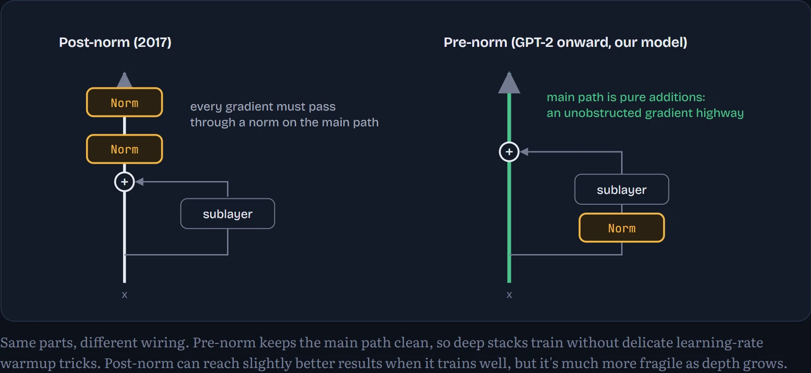
One consequence of pre-norm: the stream itself is never normalized on its way up, so it needs one final norm before the output layer. That's the lnf you'll see in the code.
Teaching a bag of letters to count
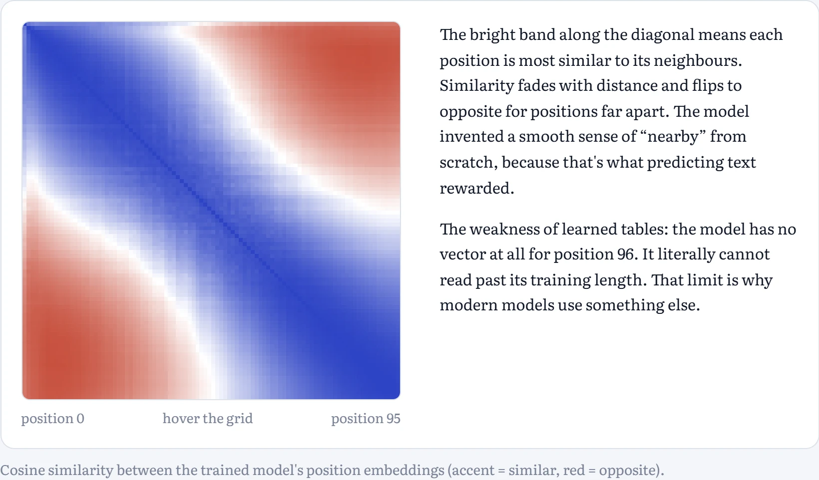
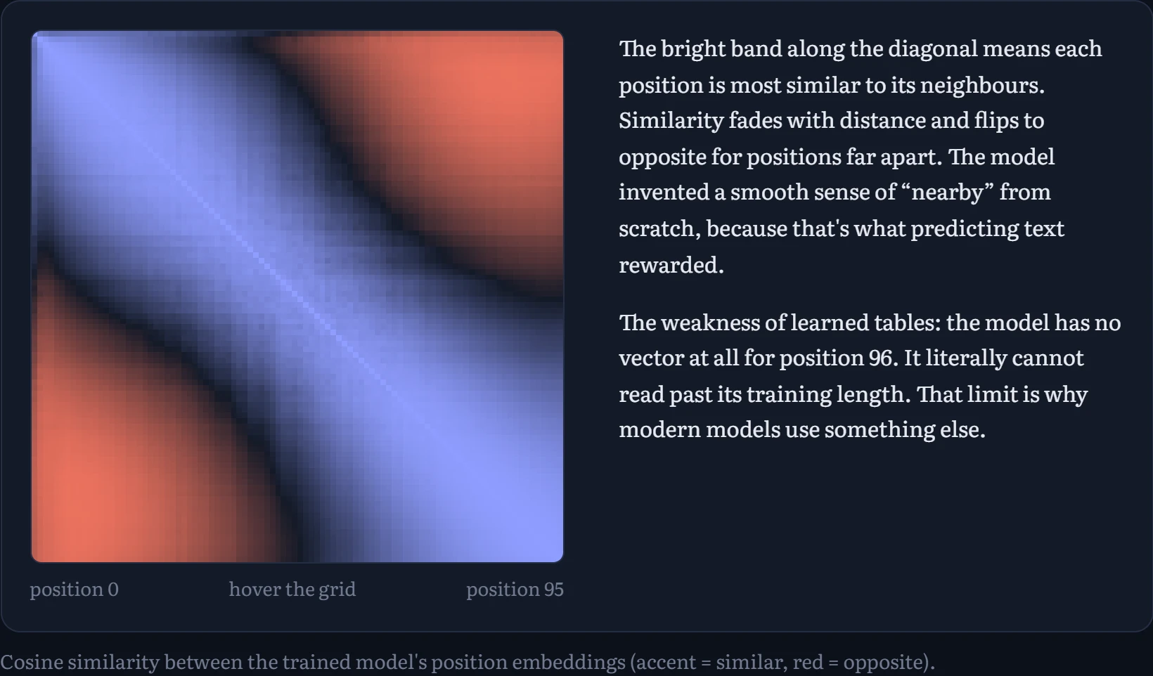
Attention compares contents, never positions. Our model solves this the simplest way: a second lookup table, wpe, with one learned vector per position (0 to 95). Before the first block, each token's vector becomes embedding of the character + embedding of the position.
Nobody told the model what positions mean. It had to learn that position 40 is “next to” 41 purely from predicting text. Did it? Here's how similar every learned position vector is to every other one, read straight out of the trained weights:
How to read it: the square compares every position with every other. The pixel in row i, column j shows how similar position i's vector is to position j's: blue means similar, red means opposite, pale means unrelated. The diagonal compares each position with itself, so it's always the brightest.
RoPE: position by rotation
Most current models use rotary position embeddings (RoPE). Instead of adding a position vector, they rotate each query and key by an angle proportional to its position.
Think of two hands on a clock that both turn at the same speed. Whatever time it is, the angle between them stays the same; only their absolute position on the dial changes. RoPE turns each word's query and key like clock hands, by an amount set by the word's position. The attention score depends on the angle between them, so it depends only on how far apart the two words are, not on where in the text they sit. Here's the mechanism in 2-D: the two positions and their score.
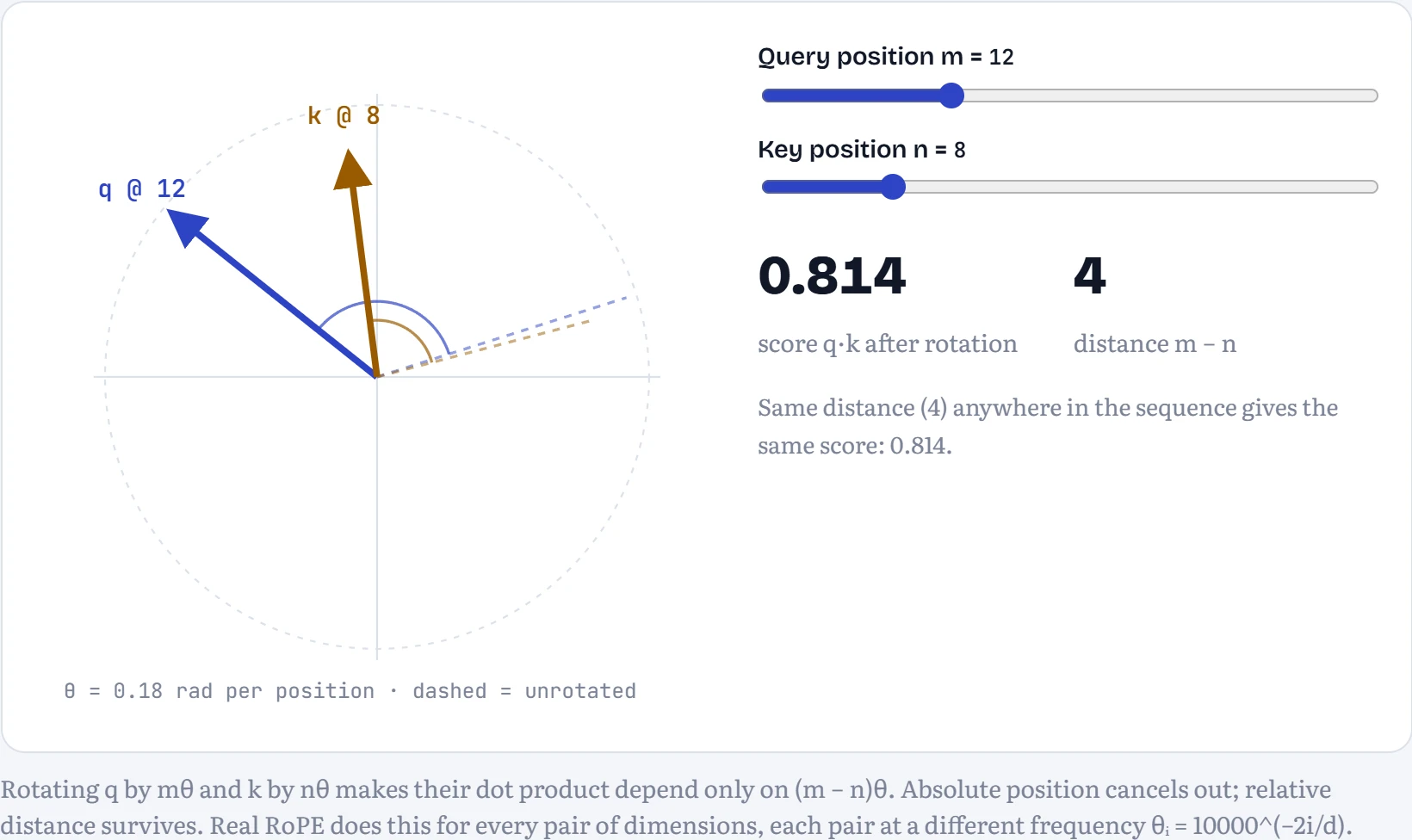
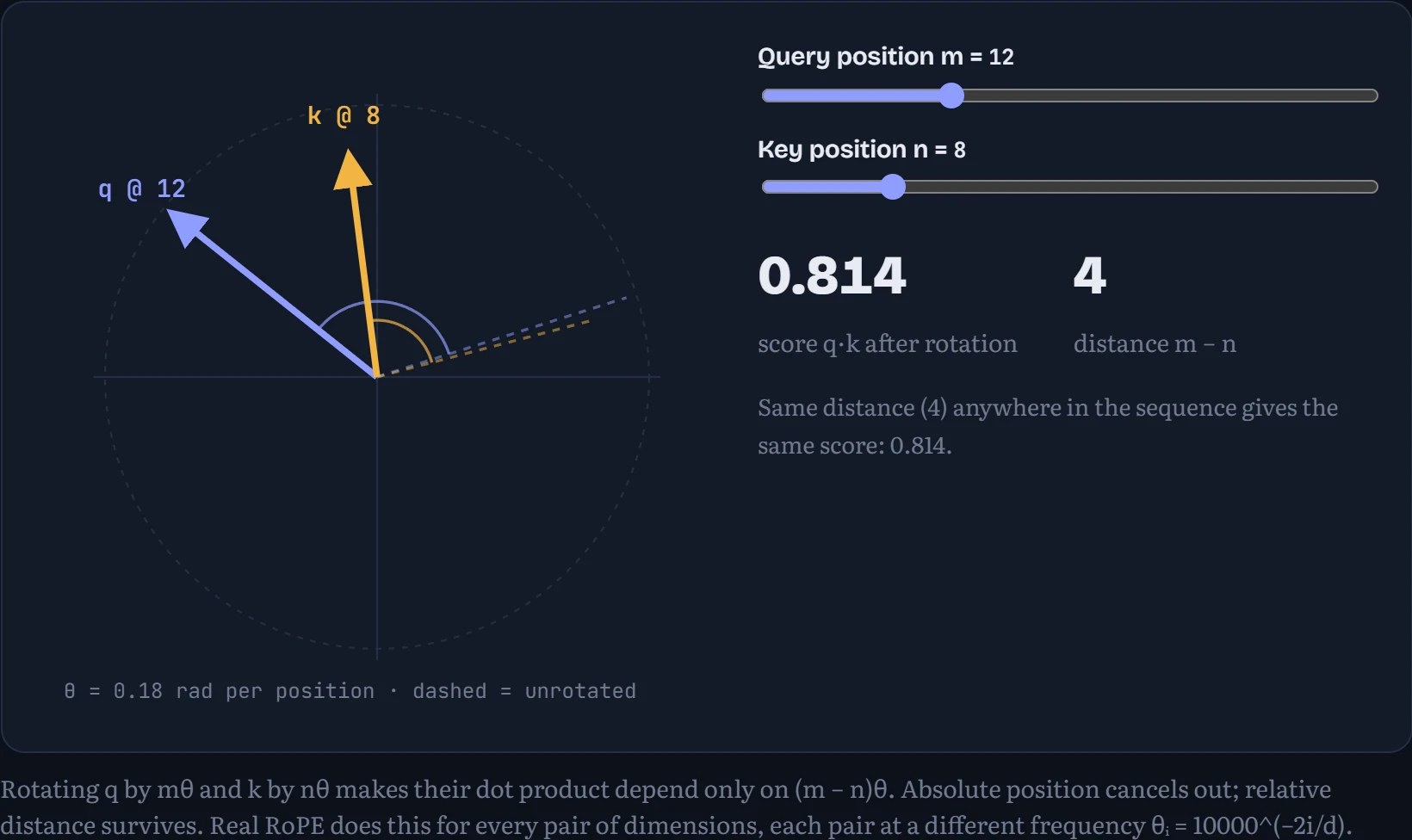
Shift both positions by the same amount and the score doesn't move. That's the whole point: “the word three back” means the same thing at position 10 and at position 10,000. It's not a free pass to infinite length, though. Models still struggle past the lengths they trained on, and techniques for stretching RoPE further are an active area (Chapter 12.3).
Five ways to encode position, tested past their training length
Learned tables and RoPE aren't the only options. The original Transformer used sinusoidal positions: a fixed pattern of sine and cosine waves at different frequencies added to each token, so every position gets a unique fingerprint with no training at all. ALiBi (Press and colleagues, 2021) adds nothing to the tokens; instead each attention score gets a penalty proportional to how far back the other token is, so attention naturally fades with distance. And some models use no position information at all, relying on the causal mask, since a token can tell roughly where it is by how many tokens it can see. I trained five small, otherwise identical Transformers on 64-character windows of TinyStories, one per scheme, then measured their loss on 256-character windows: four times longer than anything they saw in training. How to read the chart: average loss at each position (lower is better); everything right of the dashed line is longer than the training windows.
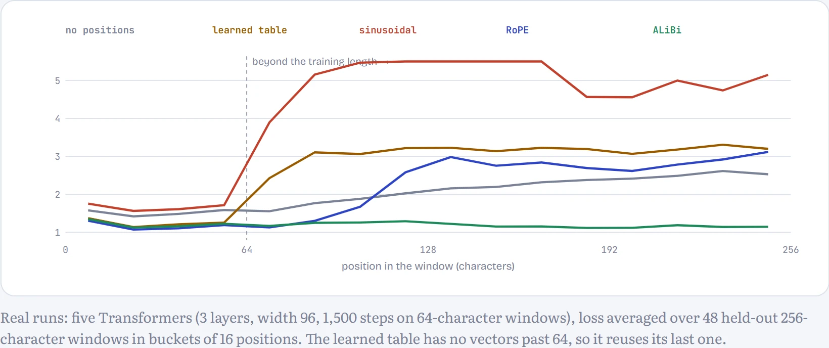
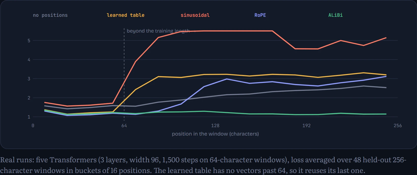
Inside the training length all five work (no positions 1.52, learned table 1.24, sinusoidal 1.66, RoPE 1.17, ALiBi 1.21). Past it, they split apart. ALiBi barely notices (1.18 on average beyond position 64): its distance penalty works the same at position 200 as at 20, and distant tokens are faded out anyway. Sinusoidal positions fall apart worst (5.25): positions past 64 produce wave patterns the model has never seen added to its inputs. The learned table, reusing its last vector, and RoPE both degrade steadily (RoPE 2.45, reaching 2.86 at the far end): RoPE's rotation angles for long distances are still unfamiliar. Even no position information extrapolates better than sinusoidal (2.19).
Two fixes, both measured. Restrict each token to attending over only the previous 64 positions, a sliding window, and RoPE stays at 1.12 all the way out, because every distance it sees is one it trained on. Position interpolation squeezes 256 positions into the range 0 to 64 by scaling the rotation angles. Without any retraining it made things worse here (3.48): it changes every distance the model learned, including the short ones that matter most for predicting the next character. That's why real models apply it together with a short fine-tune at the new length, and why refinements such as YaRN stretch only the low frequencies and leave the short-distance ones alone. Chapter 12.3 returns to this from the long-context side.
Watch the stream think
Here's an experiment you can only do because the model is right here. After each block, take the residual stream at the last position and push it through the final norm and output layer early, as if the model had stopped there. You get the model's best guess so far, layer by layer. This trick is called the logit lens. In plain words, it's like asking someone to blurt out their best guess halfway through thinking about a question, then again a bit later, and watching the answer firm up.
The table shows the top guesses for the next character after your text.
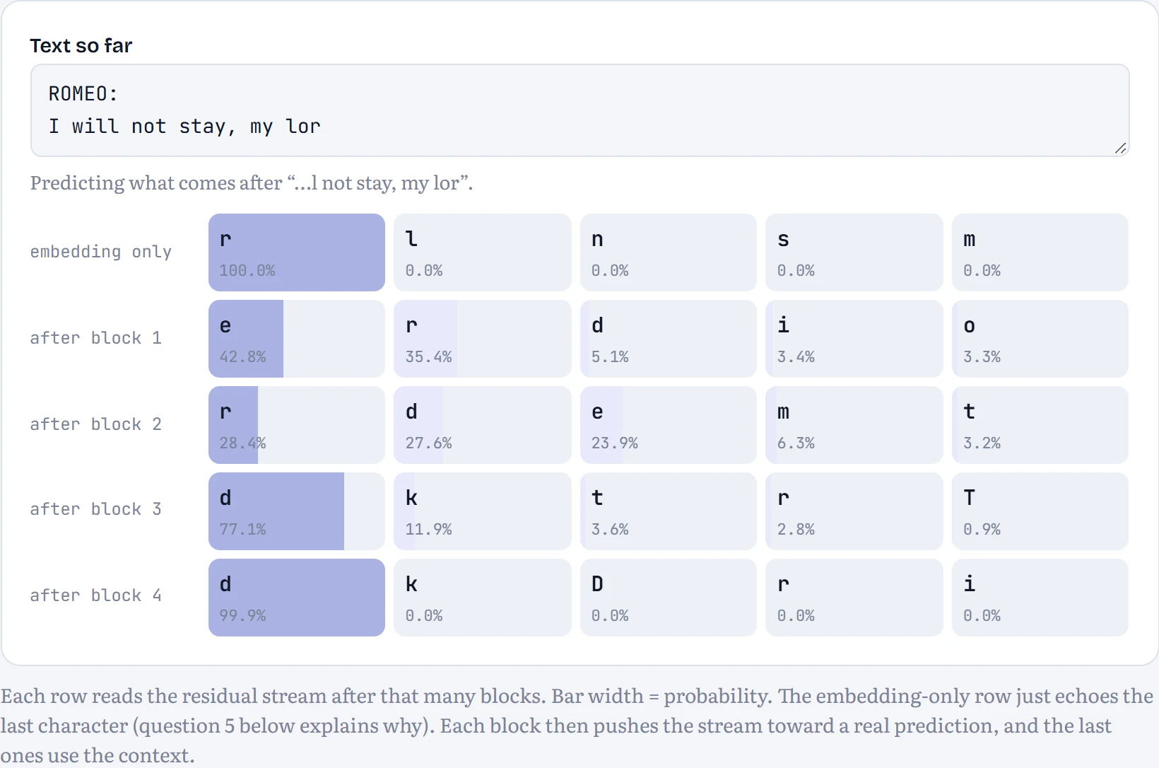
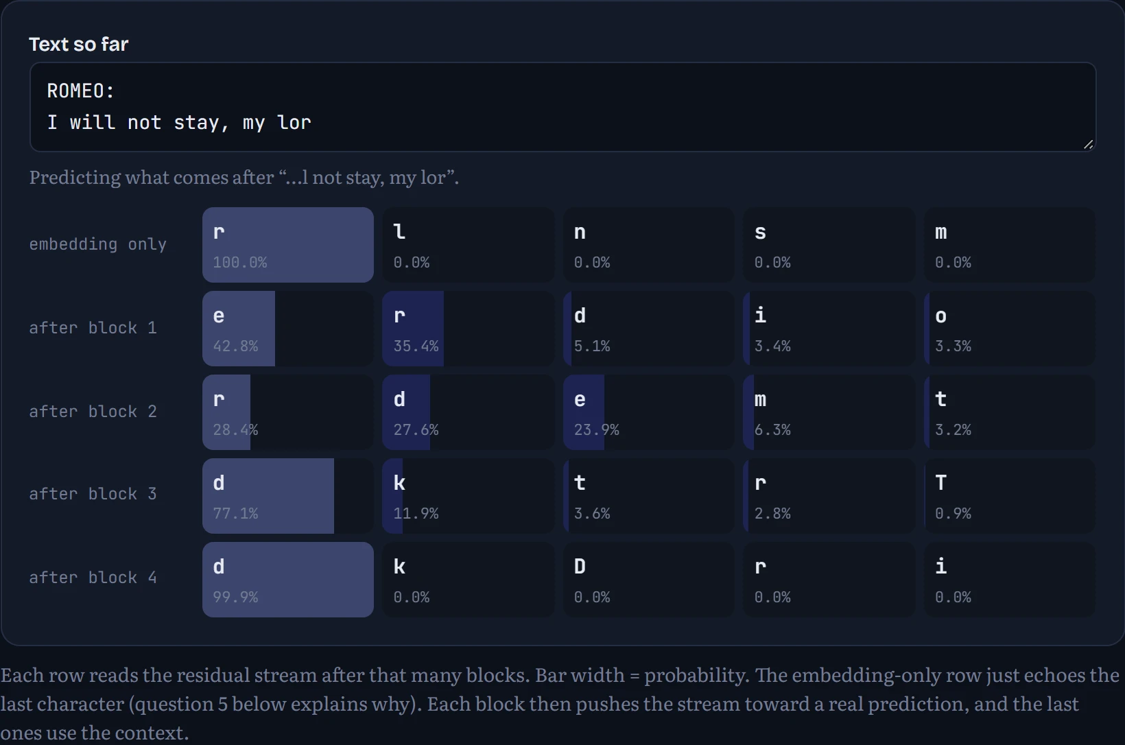
OPEN RESEARCH. The logit lens is a heuristic. Earlier layers were never trained to be read by the final output layer, so their guesses can be misleading, especially in larger models. Researchers use trained per-layer probes (the “tuned lens”) to get fairer readings.
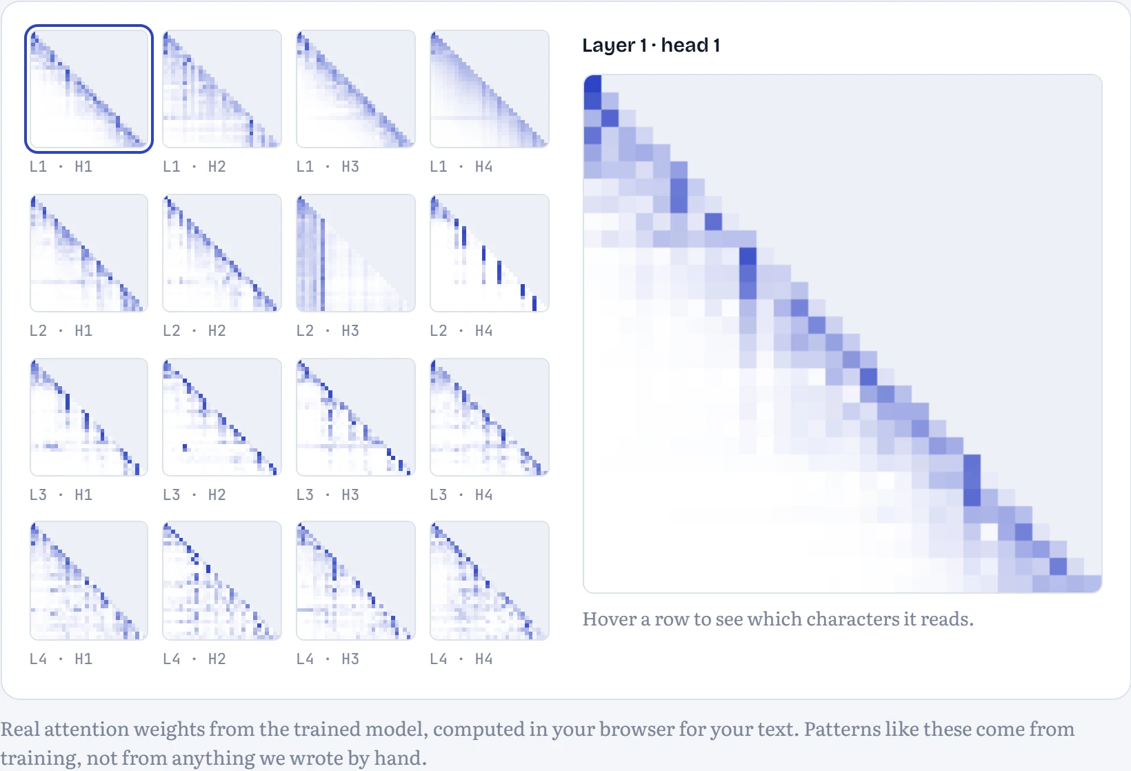
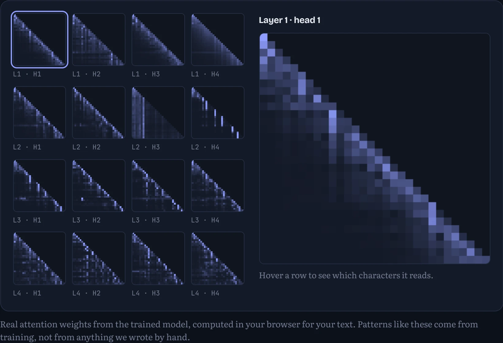
And here's every attention head, on your text
Each small square is one head's attention pattern for the last part of the text above (rows ask, columns answer; brighter = more attention). Look for heads that attend to the previous character (a bright line just under the diagonal), heads that jump back to the start of the line, and heads that seem to look for the same letter earlier on.
Continue the lesson
The whole lesson, with its drawings and its questions. 7 more sections after the ones above.