
Pre-training at scale: MinHash deduplication, Chinchilla scaling laws, bf16, ZeRO and pipeline parallelism
A base model learns one thing: predict the next token on whatever text it is fed, so most of pre-training is deciding what not to feed it. Final loss falls along a smooth power law in model size, and for a fixed compute budget there is a best balance between model size and training tokens, the Chinchilla result.
What this page answers
How does MinHash find near-duplicate documents?
It breaks each document into overlapping word groups, hashes them many ways and keeps the smallest hash each time. Two documents agree on a minimum with probability equal to their Jaccard similarity, so counting agreements estimates it. Read it in “Pre-training starts with a very large, very dirty pile of text”
What are LLM scaling laws?
Train models of different sizes the same way and their final loss falls along a smooth power law in parameter count, L(N) = E + A times N to the power minus alpha, where E is the irreducible part. Read it in “Scaling laws: loss is a power law in size”
Pre-training starts with a very large, very dirty pile of text
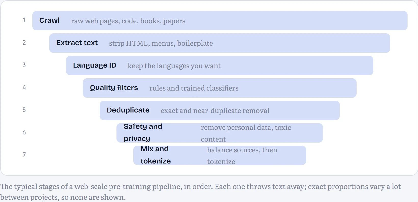
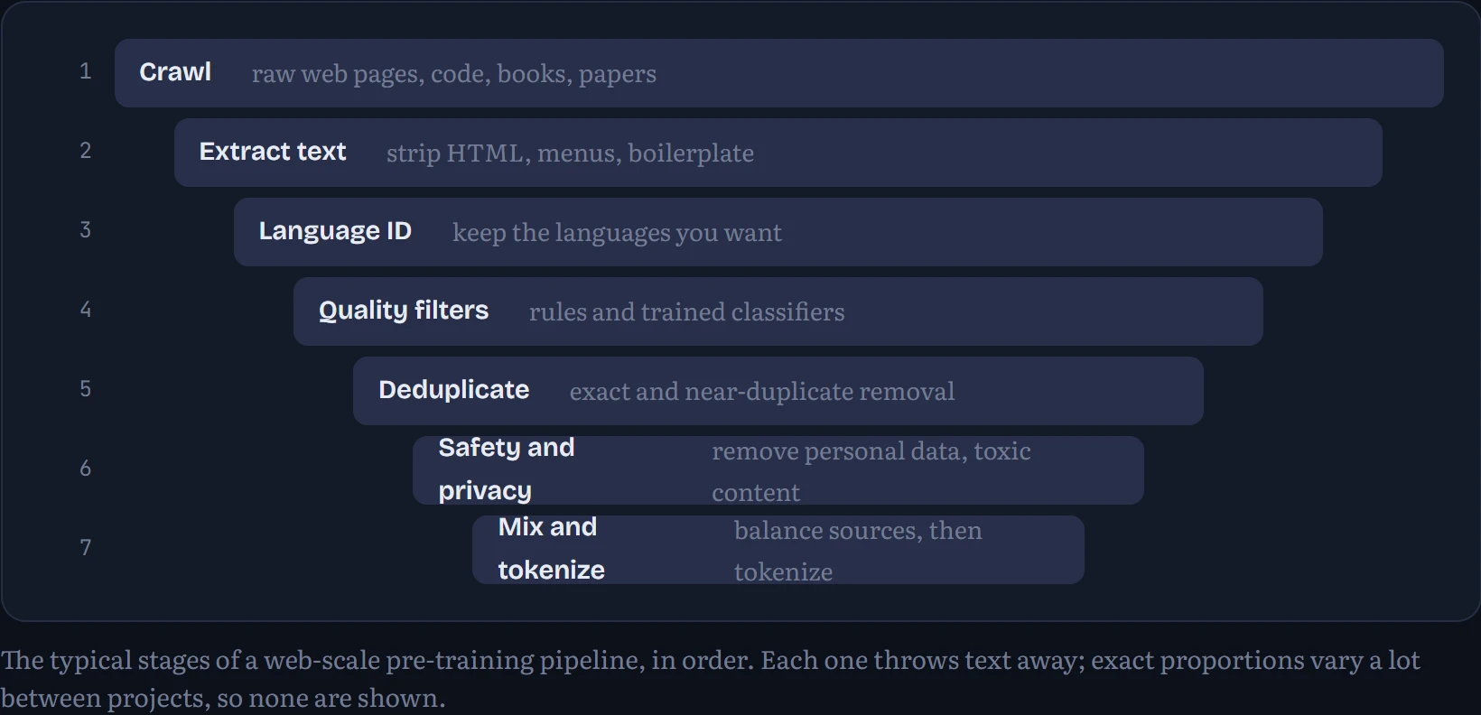
A base model learns one thing: predict the next token on whatever text you feed it. So it becomes a compressed reflection of that text, including its spam, its duplicated cookie banners and its errors. Most of the work in a real pre-training project goes into deciding what not to feed it. The usual pipeline is a funnel:
Finding near-duplicates without comparing everything with everything
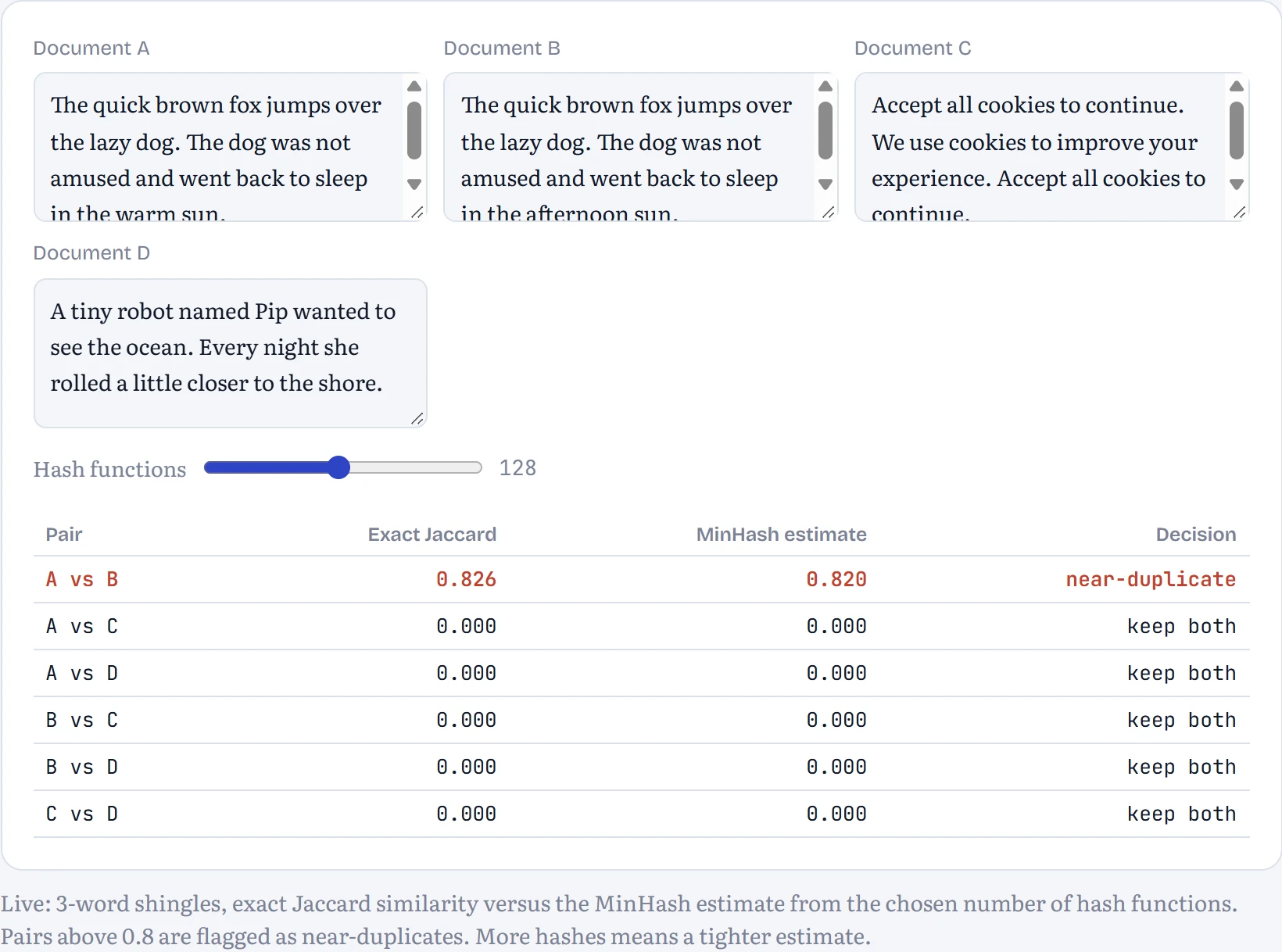
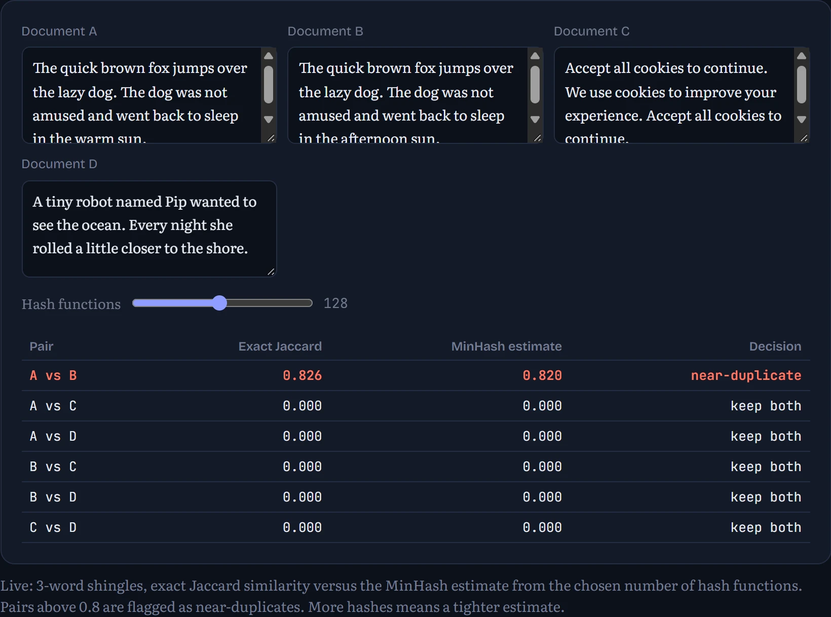
The web repeats itself constantly: mirrored articles, templated product pages, the same licence text on a million sites. Training on duplicates wastes compute and nudges models toward memorizing. But comparing every pair of documents among billions is hopeless. The standard trick is MinHash: break each document into overlapping word groups (“shingles”), hash them many different ways, and keep only the smallest hash from each. Two documents agree on a given minimum with probability exactly equal to their Jaccard similarity, the share of shingles they have in common.
Imagine every possible three-word phrase shuffled into one random order. Ask each document: “which of your phrases comes first in this shuffle?” If two documents share most of their phrases, they'll usually give the same answer; if they share few, they'll rarely agree. Repeat with 128 different shuffles and count how often they agree. That fraction is a good estimate of how much they overlap, and each document only has to remember 128 numbers instead of its whole text. That's what makes it possible to compare billions of documents. Here it is on a few documents:
Quality filters are mostly simple rules
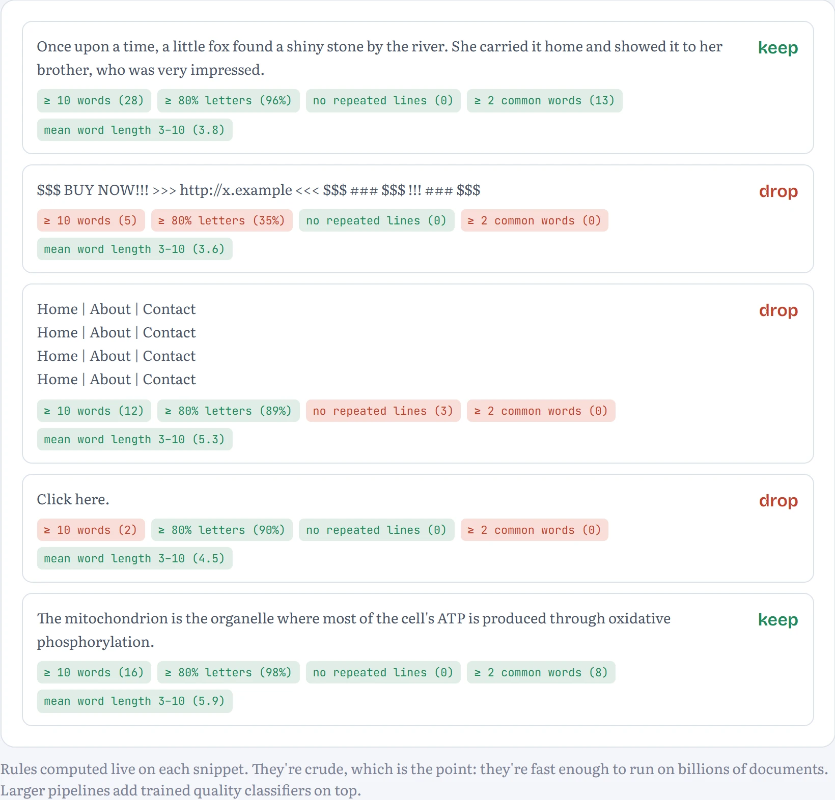
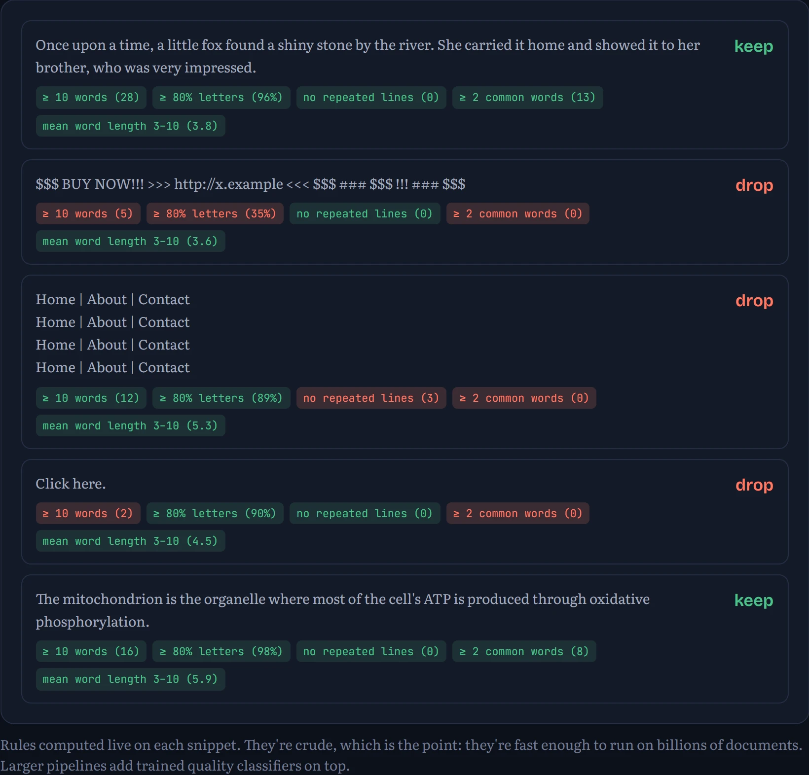
Surprisingly much filtering is done with cheap heuristics, in the spirit of the rules published with datasets like C4 and Gopher's MassiveText: drop documents that are too short, mostly symbols, full of repeated lines, or missing ordinary words. Here are a few rules running on example snippets:
Mixtures: what you feed it is what it becomes good at
Real pre-training data is a blend: web pages, code, books, papers, maths, conversations, increasingly synthetic text written by other models, and more and more of it in many languages. Choosing the proportions, the data mixture, is one of the most consequential and most secret decisions in building a model. It's a zero-sum game for a fixed budget: every token spent on one source isn't spent on another. I measured that trade-off directly. The same small model (355K parameters, 1,500 steps of 32 sequences) was trained for the same number of steps on children's stories mixed with Shakespeare in different proportions. How to read the chart: held-out loss on each kind of text (lower is better) against the share of Shakespeare in training.
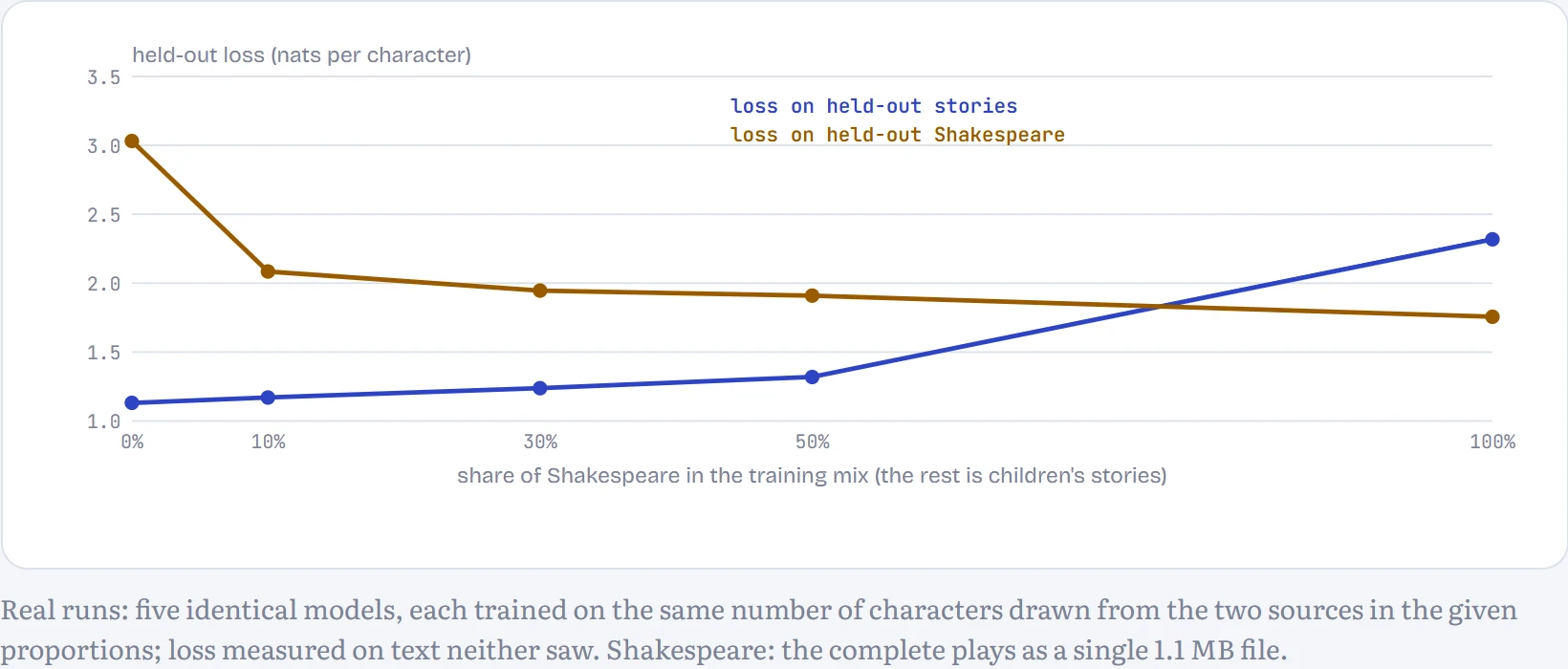
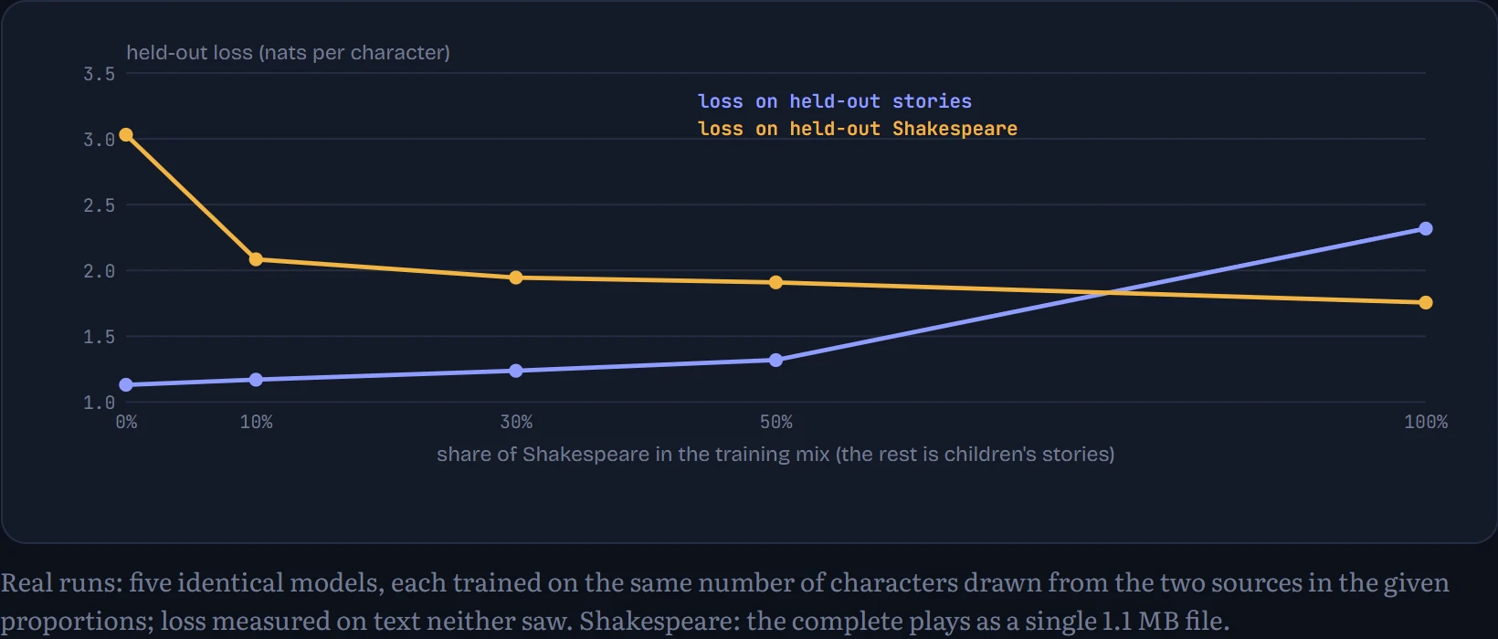
With no Shakespeare at all, the model is good at stories (1.13) and lost on Shakespeare (3.03). Spending just 10% of training on Shakespeare cuts its Shakespeare loss to 2.08, while the story loss only rises from 1.13 to 1.17. That asymmetry is the most useful fact about mixtures: the first slice of a new domain buys a lot, and a little goes a long way. At a 50/50 mix the model is fair at both (1.32 and 1.91); trained only on Shakespeare it reaches 1.76 there and is poor at stories (2.32). Frontier labs tune exactly this trade-off, with code, maths and multilingual text, by training many small models on different mixtures and fitting curves like these, then scaling up the winner.
What duplicates actually do
The MinHash demo above finds duplicates; here's why it's worth the trouble. I trained the same model on 4,100 different stories, and on a corpus where 100 of the stories appear many times (plus a planted test set, explained next), in two settings: 10 copies with 1,500 training steps, and 40 copies with 3,000 steps. Then I gave each model the first 64 characters of a story and checked whether it could continue the next 64 word for word. How to read the table: the share of stories recited exactly, the loss on the repeated stories, and the loss on held-out stories neither model saw (real skill).
| 10 copies, 1,500 steps | 40 copies, 3,000 steps | |||
|---|---|---|---|---|
| clean | with duplicates | clean | with duplicates | |
| Recites a repeated story word for word | 0% | 0% | 0% | 0% |
| Loss on the repeated stories | 0.952 | 0.893 | 0.754 | 0.574 |
| Loss on held-out stories (real skill) | 1.147 | 1.144 | 0.976 | 1.054 |
Neither setting made this small model recite a repeated story word for word: 64 characters in a row, exactly right, is a high bar for 355K parameters. But the memorizing shows clearly in the loss. On the repeated stories it fell 6% below what the clean model scored on the same stories at 10 copies, and 24% below at 40 copies: the model was learning those particular stories, not stories in general. Larger models memorize far more readily: studies of GPT-style models found that the amount of text they can reproduce verbatim grows with model size and with how often a passage is duplicated in training (Carlini and colleagues, 2023). That's how models end up reproducing copyrighted text or personal data, and deduplication is the first line of defence. With 10 copies, general skill barely moved (held-out loss 1.147 clean against 1.144 with duplicates). With 40 copies it clearly hurt: held-out loss rose from 0.976 to 1.054, because most of the training documents were now copies, and every step spent re-reading them was a step not spent on new stories. Duplication costs twice: more memorization, less learning.
Contamination: when the test leaks into training
The same duplicated corpus hid one more thing: 50 stories from a “benchmark” set, ten copies each. The other 50 benchmark stories were kept out. If you judged that model on the leaked half, you'd be measuring memory, not skill. How to read the chart: the model's loss on benchmark stories it was trained on, against benchmark stories it never saw, for both training runs.
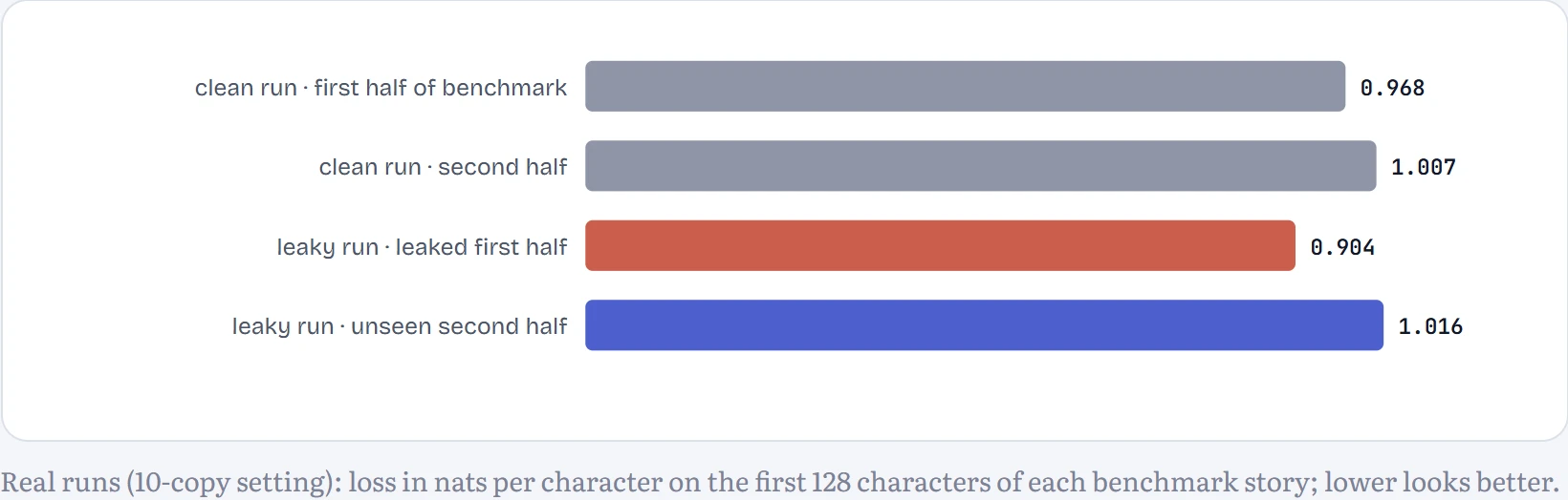
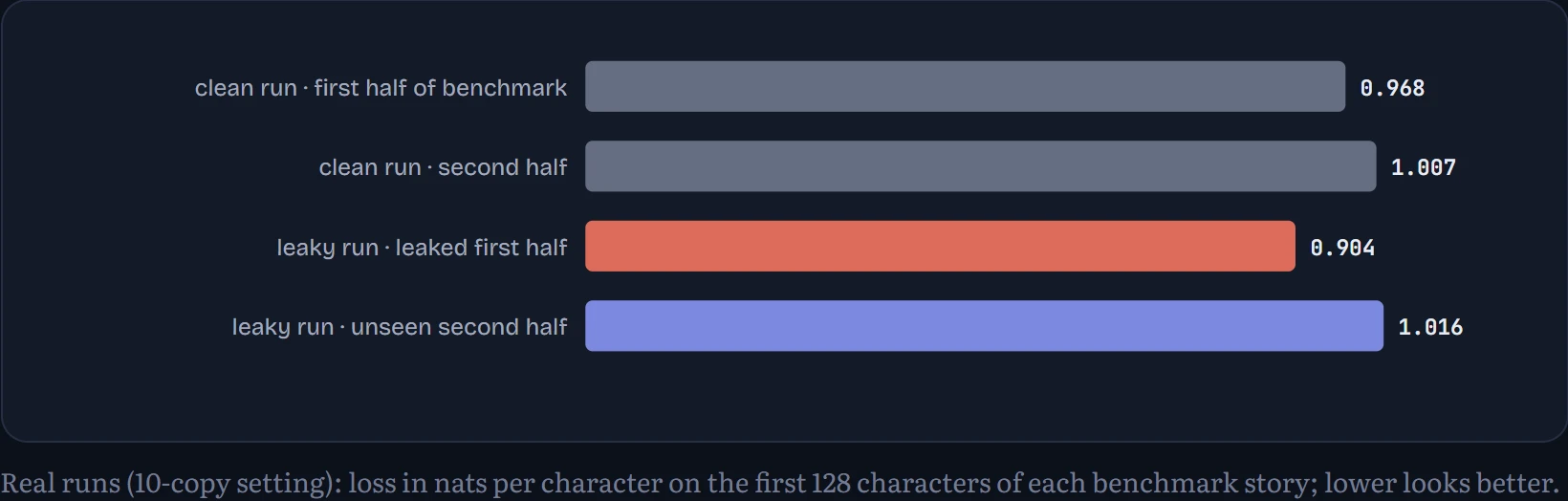
Even without any leak, the two halves of the benchmark aren't equally hard: the clean model scored 4% lower loss on the first half than the second. That's the baseline to compare against. In the leaky run the leaked half scored 11% lower than the unseen half, so leaking added roughly 7 percentage points of flattering advantage; with 40 copies the gap grew to 34% (against 3% for the clean model). A benchmark score from a contaminated model measures partly memory, not skill, and the inflation grows with repetition. Labs guard against it by searching training data for benchmark text (n-gram overlap checks) and by keeping private, freshly written test sets; Chapter 15 shows how dramatically contamination can inflate an exact-match score.
FOR OUR EXPERIMENTS. We skip all of this by using TinyStories, a synthetic dataset of short children's stories written by a language model to be simple and clean (Eldan and Li, 2023). It's ideal for small models because it contains so little noise. I used its 22.5 MB validation file as our whole corpus, kept plain ASCII characters, and held out the last 5% for measuring loss.
What a base model learns, and what “emerges”
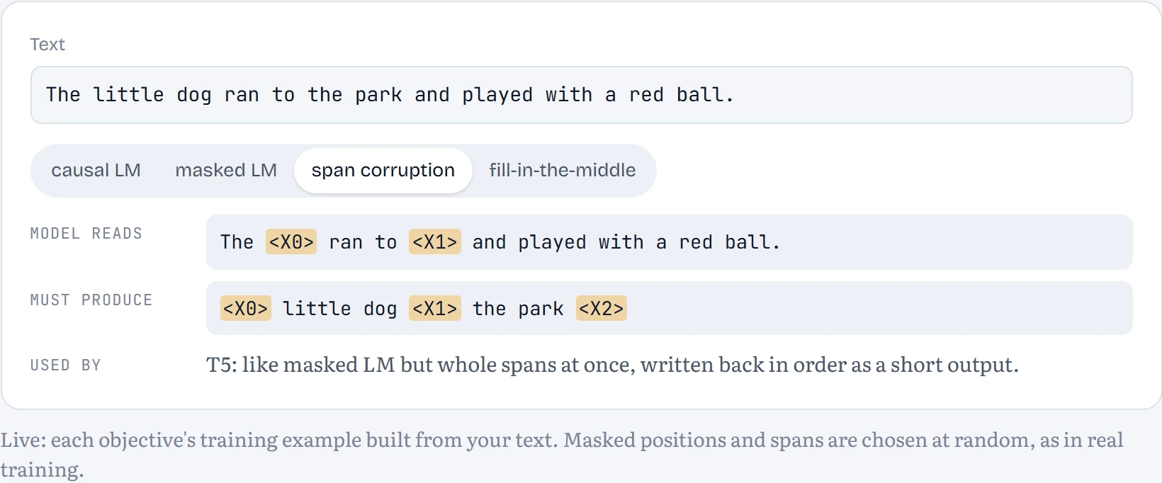
There are a few ways to set up the prediction task. Causal LM predicts each next token from the ones before (GPT, your mini-GPT). Masked LM hides random tokens and predicts them from both sides (BERT). Fill-in-the-middle, used for code models, cuts a document into prefix, middle and suffix, then moves the middle to the end, so an ordinary causal model learns to fill gaps, which is exactly what code completion inside a file needs.
As models scale, people observe abilities that small models seem to lack entirely and large ones suddenly have: multi-digit arithmetic, some kinds of reasoning. These were called emergent abilities. Here's a reason to be careful with that word. Suppose a model's per-token accuracy improves smoothly with scale. A task scored as all-or-nothing on a k-token answer succeeds with probability pᵏ.
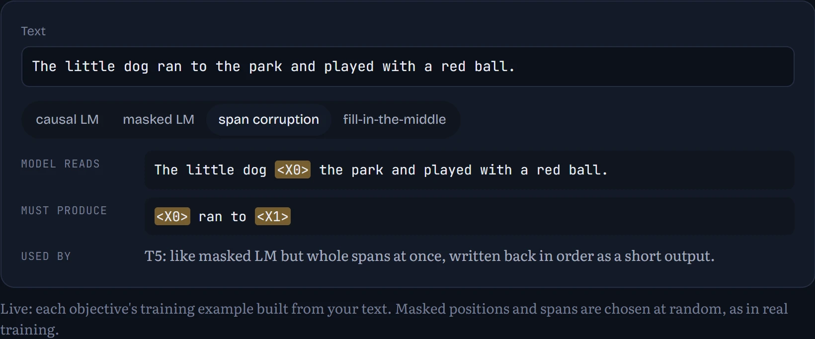
A fourth objective sits between causal and masked: span corruption, used to train T5 (Raffel and colleagues, 2019). Whole stretches of text are cut out and replaced by placeholder markers, and the model learns to write back the missing pieces in order. In the figure: one sentence, and the training example each of the four objectives makes from it: what the model reads, and what it must produce.
Think of adding two 10-digit numbers, where the answer only counts if every digit is right. Get each digit right 90% of the time and the whole answer is right only 0.9¹⁰ ≈ 35% of the time. Improve to 99% per digit and whole answers jump to about 90%. The model got a little better at each digit, steadily; the score for whole answers makes it look as if a new skill suddenly appeared. The chart shows exactly that effect:
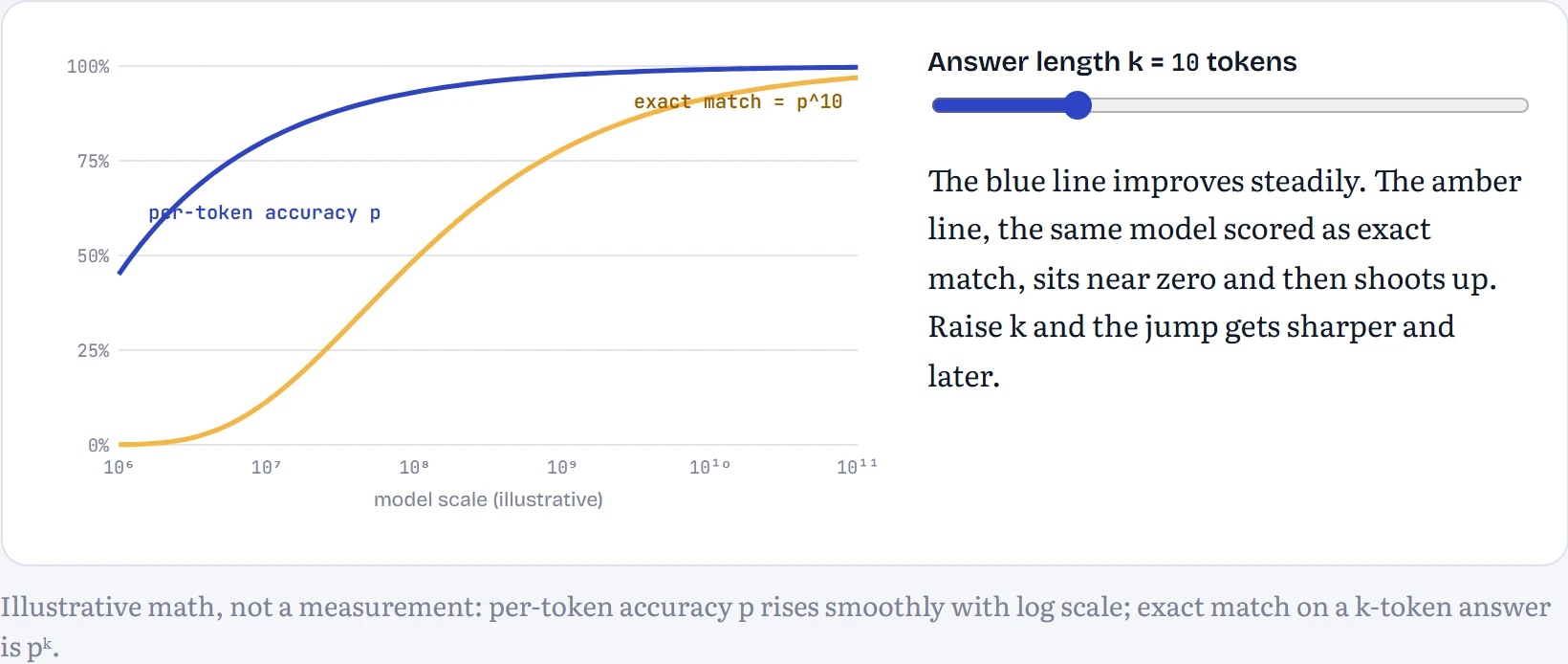
OPEN RESEARCH. Schaeffer and colleagues (2023) argued that many reported emergent abilities are artefacts of all-or-nothing metrics like this one, and become smooth under continuous metrics. Others point to tasks that still look abrupt under fair metrics. Whether, and in what sense, capabilities emerge discontinuously is unsettled. What's not in doubt is that the underlying loss improves smoothly and predictably, which is what the rest of this lesson is about.
Scaling laws: loss is a power law in size
Train models of different sizes the same way and plot their final loss against parameter count on a log scale, and you get a remarkably smooth curve. Kaplan and colleagues (2020) found it across seven orders of magnitude, and it has a simple form:
L(N) = E + A · N−α
N is the number of non-embedding parameters (embedding tables behave differently, so they're left out by convention). E is the loss you'd approach with an infinitely large model on this data and budget: the irreducible part, partly the genuine randomness of text. A and α describe how fast you get there.
The formula says a model's loss has two parts. There's a floor (E) that no amount of extra size will push below, at least with this data and this training budget. And there's a part that shrinks as the model grows (A·N−α). α is how fast it shrinks: with our α of 0.29, every doubling of model size cuts that shrinking part by about 18%. So each doubling helps, but each helps a little less in absolute terms than the last.
What does a loss number mean? It's measured in nats per character, and eloss turns it into something you can picture. The smallest model's 1.92 means that, on average, it's as unsure as if it were picking between about 7 equally likely next characters. The biggest model's 1.09 is like picking between about 3.
Here's what our sweep produced:
| Width d | Non-embedding params N | Tokens seen | Training FLOPs | Final validation loss | Law's fit | Time |
|---|---|---|---|---|---|---|
| 16 | 13,152 | 4.1M | 3.2×10¹¹ | 1.922 | 1.914 | 74 s |
| 24 | 28,944 | 4.1M | 7.1×10¹¹ | 1.652 | 1.667 | 75 s |
| 32 | 50,880 | 4.1M | 1.3×10¹² | 1.539 | 1.522 | 54 s |
| 48 | 113,184 | 4.1M | 2.8×10¹² | 1.350 | 1.353 | 2 min |
| 64 | 200,064 | 4.1M | 4.9×10¹² | 1.242 | 1.254 | 5 min |
| 96 | 447,552 | 4.1M | 1.1×10¹³ | 1.147 | 1.140 | 8 min |
| 128 (predicted, then trained) | 793,344 | 4.1M | 1.9×10¹³ | 1.086 | 1.073 | 6 min |
Reading the table: a FLOP is one arithmetic operation, a single multiplication or addition. The “Training FLOPs” column is how much arithmetic each training run cost in total. “Law's fit” is what the formula says each model should have scored, so you can compare it with what it really scored.
The fit gives α = 0.29 and a floor of E = 0.71 nats per character, and every one of the six points sits within 0.017 of the curve. Kaplan's paper found α ≈ 0.076 for loss versus parameters in its setup. Ours is much steeper, and it should be: our models are tiny, each gets a fixed and modest token budget, and the floor E here belongs to this budget and data, not to language in general. Exponents depend on the setup; what transfers is the method. Each doubling of N buys a predictable, shrinking improvement.
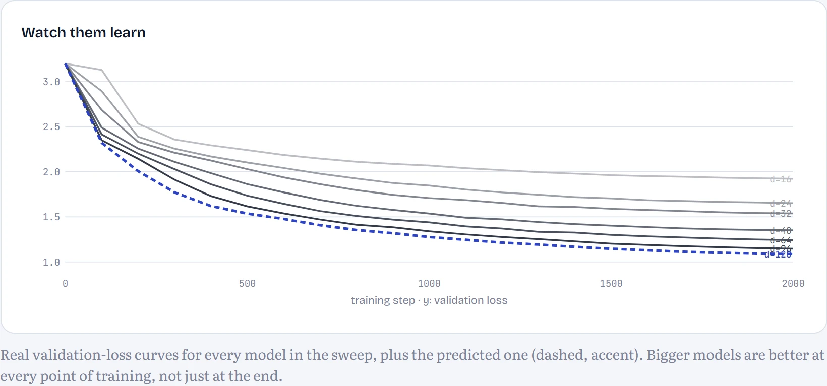
The samples tell the same story in words. Here's the smallest and the largest model writing a story, same random seed:
d = 16 · 13K parameters · loss 1.92
"Yuay, dou lige the named sarid, dig net she. He tomar sthe smome wen. The thas was wand wor itis finth law few. Onay a fon grim helilt's the fandens ien thid, the "Youm dancer lom saled, and. "hayy, they betized took the yor and mury poul. The ot athed tathere bars she verour soun. Tom ue the spirs to verom. Tim
d = 128 · 793K parameters · loss 1.09
Once upon a time, in a drawith night, there water a big bird. Tim wanted to see the restore. He was relar friends to play with her mom. She was a excited to fix her mom. In can look always so we come the rands with a man, you can my beloo. The boy notter and reborrove to her bigger too. The cat played in the mouse.
Same compute, different shapes: the Chinchilla experiment
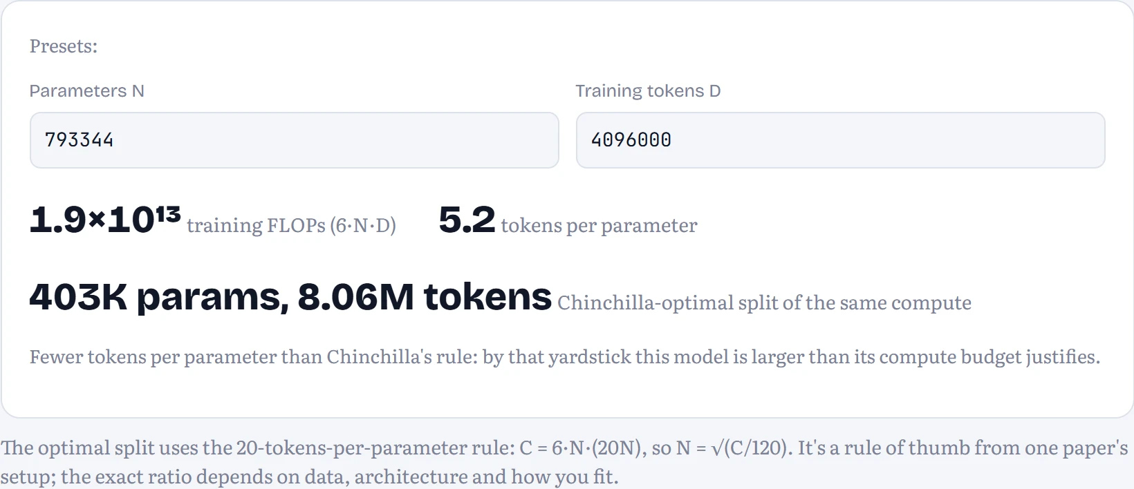
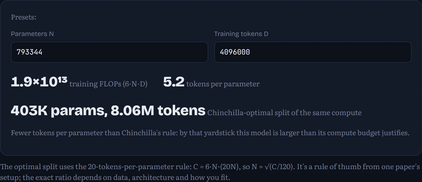
The sweep above gave every model the same number of tokens, so bigger models also cost more compute. But the real question a lab faces is different: I have a fixed compute budget. Should I train a big model on fewer tokens or a small model on more? Training costs about 6 × N × D FLOPs (Chapter 9.4), so at a fixed budget, doubling N halves D.
Why 6 × N × D? For every token of text, each parameter does one multiplication and one addition on the way forward (2 operations), and about twice that on the way back while learning (4 more). So N parameters times D tokens times 6.
The trade-off is like preparing for an exam with a fixed number of hours. A student with an enormous memory who only has time to read one chapter does badly. So does a student who races through the whole library but can only hold a little of it. Somewhere in between, memory and reading are balanced, and that's the best use of the hours. In a model, memory is parameters (N) and reading is training tokens (D).
Predict first. We trained six sizes on exactly the same compute budget each. The smallest saw the most tokens; the largest saw very few. Which wins?
- The biggest: size is everything
- The smallest: data is everything
- Something in the middle
Answer. Something in the middle. The best of the 7 was d = 24 (29K parameters on 16M tokens, about 541 tokens per parameter), with a loss of 1.344. The smallest model had plenty of data but too little capacity; the largest had capacity but saw too little text. A parabola fitted to the 5 runs nearest the bottom puts the optimum near 59K parameters and 7.62M tokens, about 128 tokens per parameter.
That ratio is not Chinchilla's 20, and it shouldn't be expected to match: our models are tiny, character-level and trained for minutes. The shape is the result that transfers: at a fixed budget there is a best size, and both extremes waste compute.
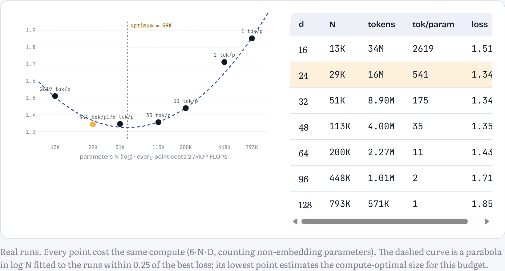
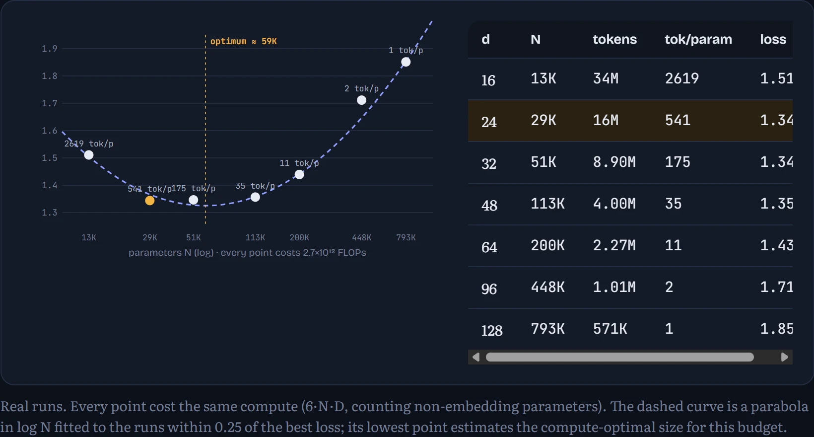
Hoffmann and colleagues (2022) ran this experiment at real scale and found that, for their setup, parameters and tokens should grow together, about 20 tokens per parameter. Their 70-billion-parameter Chinchilla, trained on 1.4 trillion tokens, beat the 280-billion-parameter Gopher trained on the same compute. Many earlier models were too big for their data.
Then practice drifted the other way, for a good reason: compute-optimal for training isn't optimal for using a model. A smaller model trained far past 20 tokens per parameter is a little worse than the compute-optimal one but much cheaper every time it answers a question. Meta's 8-billion-parameter Llama 3 was trained on over 15 trillion tokens, nearly 2,000 per parameter.
Continue the lesson
The whole lesson, with its drawings and its questions. 8 more sections after the ones above.