
Scaled dot-product self-attention: queries, keys and values, causal masking, multi-head attention and the KV cache
Self-attention lets every token find the tokens relevant to it, wherever they are, and pull their information over. Each token plays three roles: a query asking, a key describing itself and a value to hand over. Scores are scaled by the square root of the key size, masked so no token sees the future, and softmaxed into weights.
What this page answers
What are queries, keys and values in attention?
Three vectors made from each token by three learned matrices. The query says what the token is looking for, the key says what it offers to be found by, and the value is the information it hands over. Read it in “Every word plays three roles at once”
Why divide attention scores by the square root of the dimension?
A dot product of two random vectors of length d with spread 1 has a typical size of the square root of d, so scores grow as vectors get longer. Dividing by the square root of d cancels that growth and keeps the scores around size 1. Read it in “The square root nobody puts on a poster”
The problem your Chapter 7 model couldn't solve
Your mini_lm v1 read a fixed window. It glued, say, eight token embeddings end to end and pushed the result through an MLP. Slot 1 had its own weights, slot 2 had its own weights, and so on.
Now read this: “The cat sat on the mat because it was tired.” To predict anything sensible after “it”, a model has to know that “it” is the cat. Move “cat” two words earlier and the meaning is the same, but a completely different set of weights now handles it. Your MLP has to learn the cat-to-it relationship separately for every distance “cat” might appear at. That's a lot of redundant learning, and it stops dead at the edge of the window.
Predict first. Forget neural networks for a second. If you were writing the rule by hand, what would you want the model to do when it reaches “it”?
Answer. Something like: from wherever I am, go find the words that are relevant to me, wherever they are, and pull their information over. The lookup should depend on what words say, not on which slot they occupy. Keep that sentence in your head. The rest of this lesson turns it into arithmetic.
A lookup that can be wrong gracefully
You already know one kind of lookup: a Python dictionary. You hand it a key, and it either finds an exact match or throws a KeyError. That's useless for learning. Nudge the key a tiny bit and the result doesn't change at all, until suddenly it changes completely. There's no slope to follow, so gradient descent has nothing to work with.
So let's make a softer one. Give each word a vector that says what it's looking for, and each candidate word a vector that describes it. Then:
1. Score every candidate with a dot product (Chapter 2: big when two vectors point the same way).
2. Turn the scores into weights that add up to 1, using softmax (Chapter 3).
3. Return a weighted average of what each candidate carries.
The figure below shows all three steps at once for one query arrow.
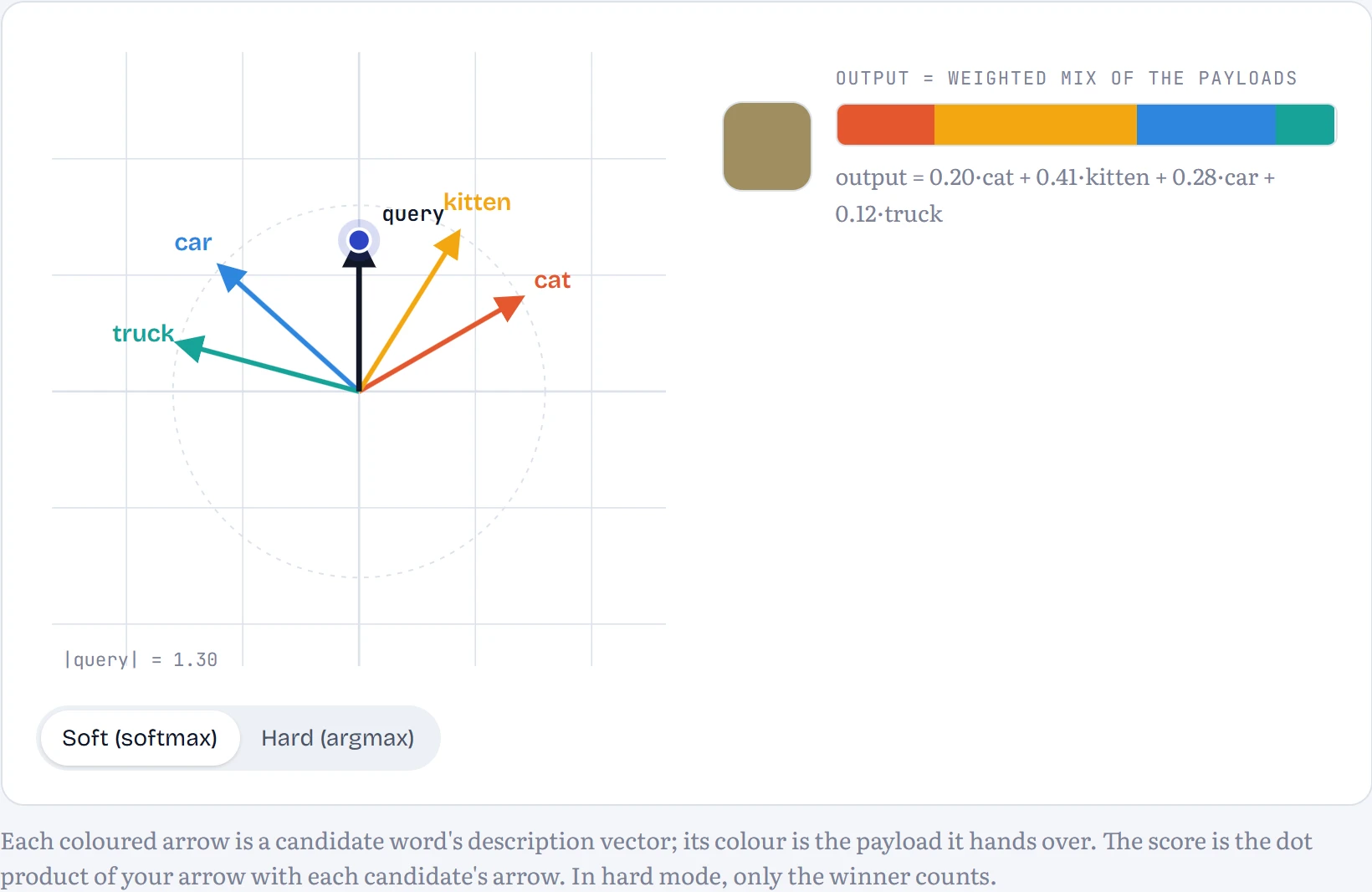
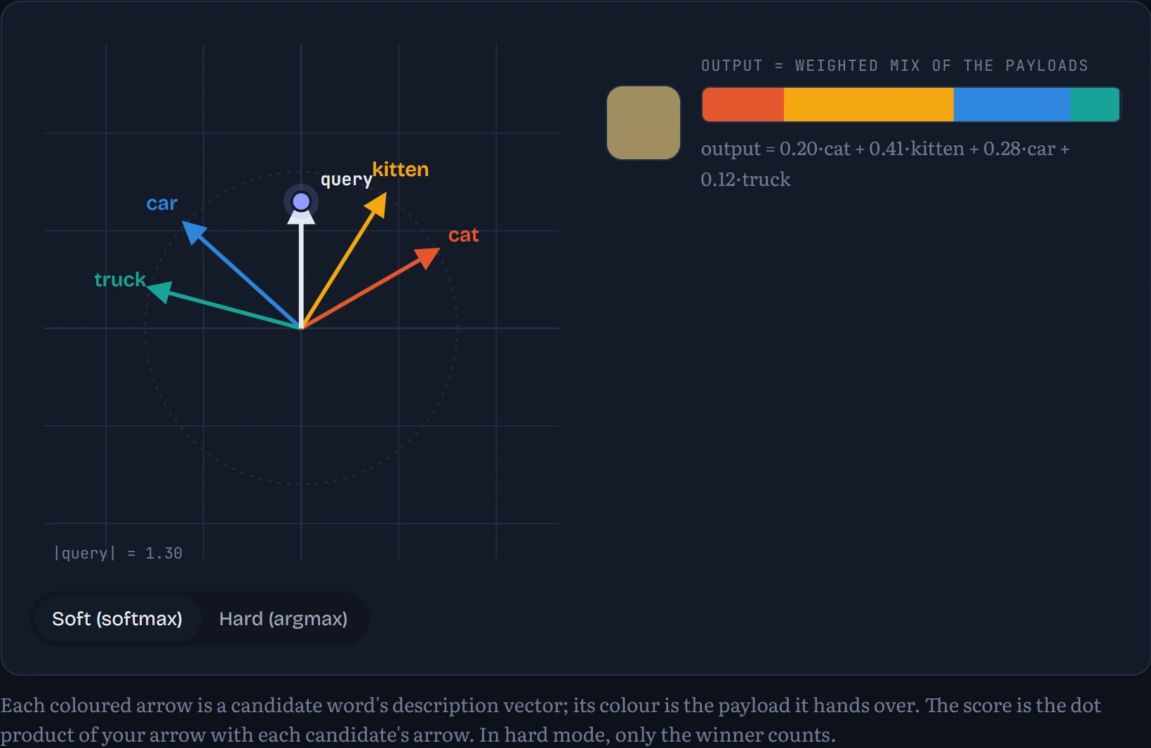
Three things are worth noticing:
Closer direction, bigger share. Pointed toward the animals, the output turns warm. Pointed toward the vehicles, it turns blue. Pointed between them, it gives a blend, which is exactly what you want when you're unsure.
Length acts like confidence. A long arrow makes every score bigger, and softmax exaggerates differences between big numbers, so the winner takes almost everything. A short arrow gives a blurry, even split. “Point at nothing” zeroes every score, and softmax of all-zeros is a perfectly flat 25% each. Softmax is a polite argmax: it picks a winner but hands everyone else a participation trophy.
The output never leaves the range of the payloads. Every weight is positive and they add up to 1, so the output is always a blend of what's already there. Attention can move information around. It can't invent new information on its own. Something else has to do that, and we'll meet it in a few sections.
In hard mode, where only the winner counts, moving the query slowly changes nothing for a while. The output stays frozen, then jumps. That flat-then-cliff shape is why we use the soft version: the slope is zero almost everywhere, so a model could never learn where to point.
Time to name things. The dark arrow is the query . The candidates' description arrows are keys. The payloads are values. The names come from databases, and for once the jargon is exactly right.
Every word plays three roles at once
In self-attention, every token is a querier and a candidate at the same time. Each token starts as one embedding vector x (from your embedding table in Chapter 6). The model then multiplies that same x by three different learned matrices:
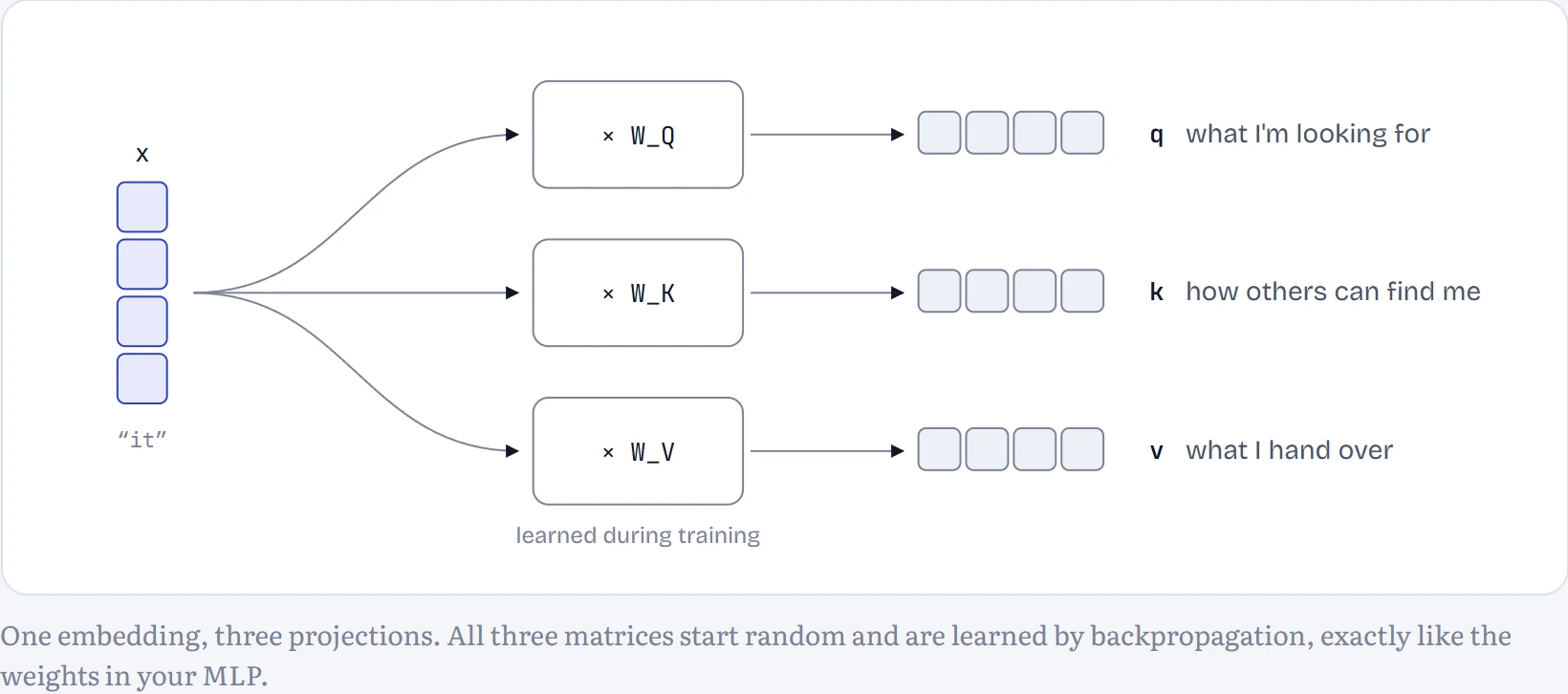
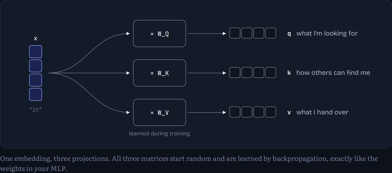
Predict first. Why bother with three matrices? What would go wrong if every token just used its raw embedding x as its query, its key and its value?
Answer. Every word would mostly attend to itself. The dot product of a vector with itself is its squared length, which is usually the biggest score in the room. You'd have a very expensive way of doing nothing.
There's a deeper reason too. What “it” is looking for (an animate noun) is not what “it” is. And what makes “cat” findable (being a noun) is not the same as what's useful to copy from it (that it's a furry animal that can be tired). Separate projections let those three jobs specialize. They also make attention directional: q_it · k_cat can be large while q_cat · k_it is small.
The whole computation, with real numbers
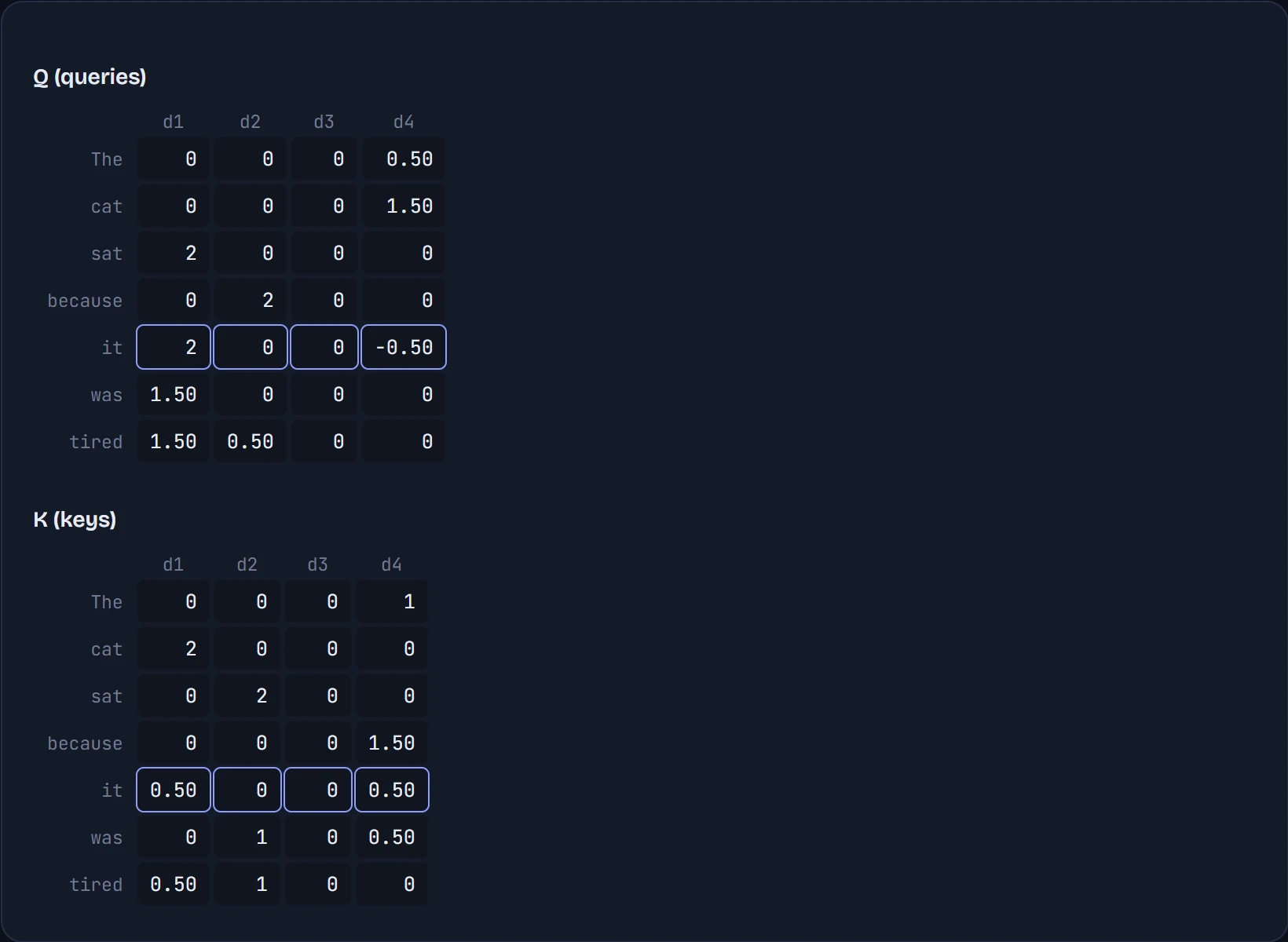
Here's the sentence from the top of the page, with tiny 4-number vectors so you can check every value by hand. I picked these Q, K and V numbers myself so the pattern is easy to read. A trained model learns its own, and they're rarely this tidy. The arithmetic is exactly what a real model does.
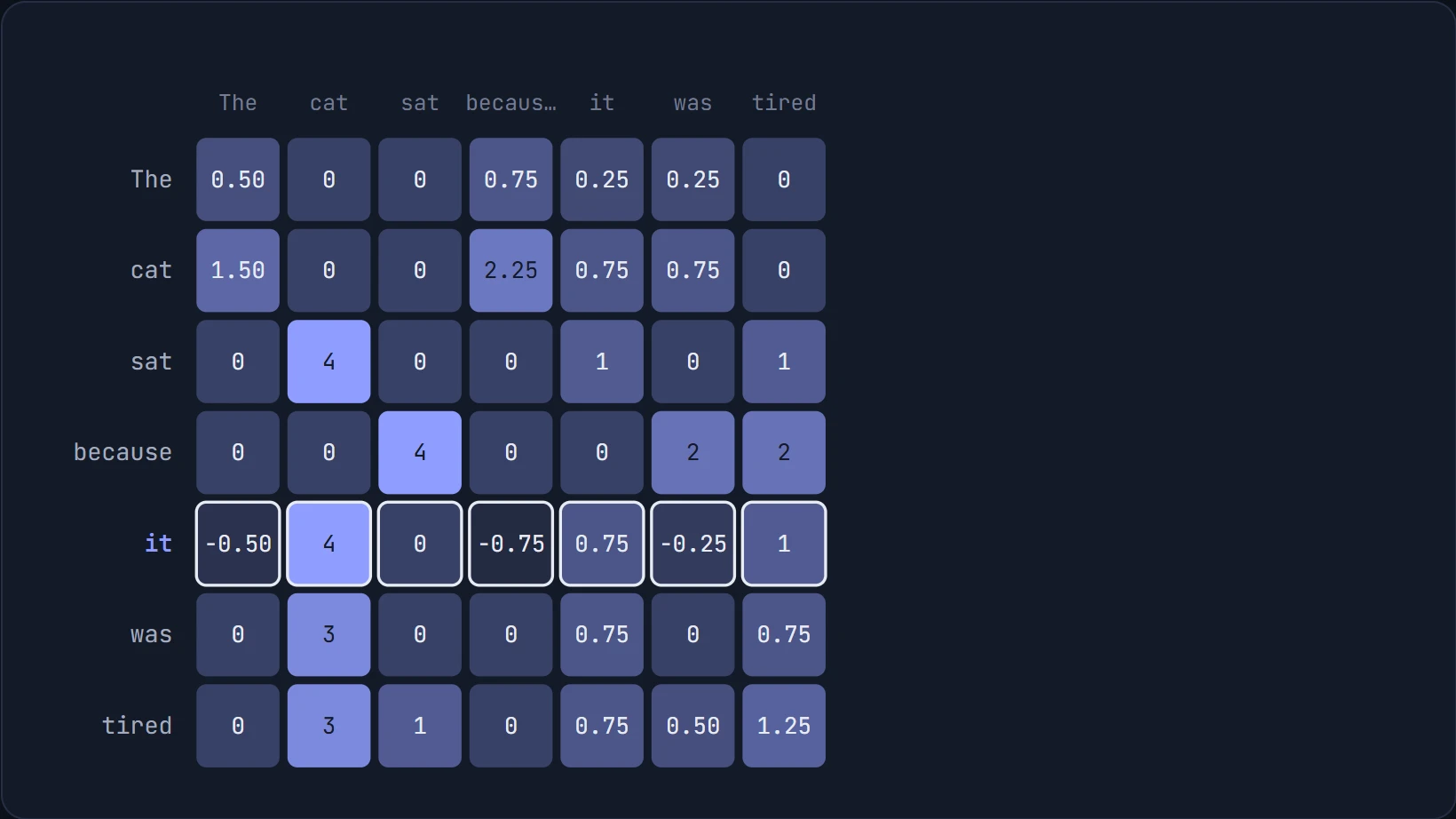
How to read the grid: each row is a word asking “who should I look at?”, and each column is a word being considered. The number in a cell is how strongly that row's word matches that column's word, and darker cells are stronger matches. The six steps transform these raw scores, one operation at a time, into the final attention weights, then use them to mix information. The explanation under each picture says what that step does.
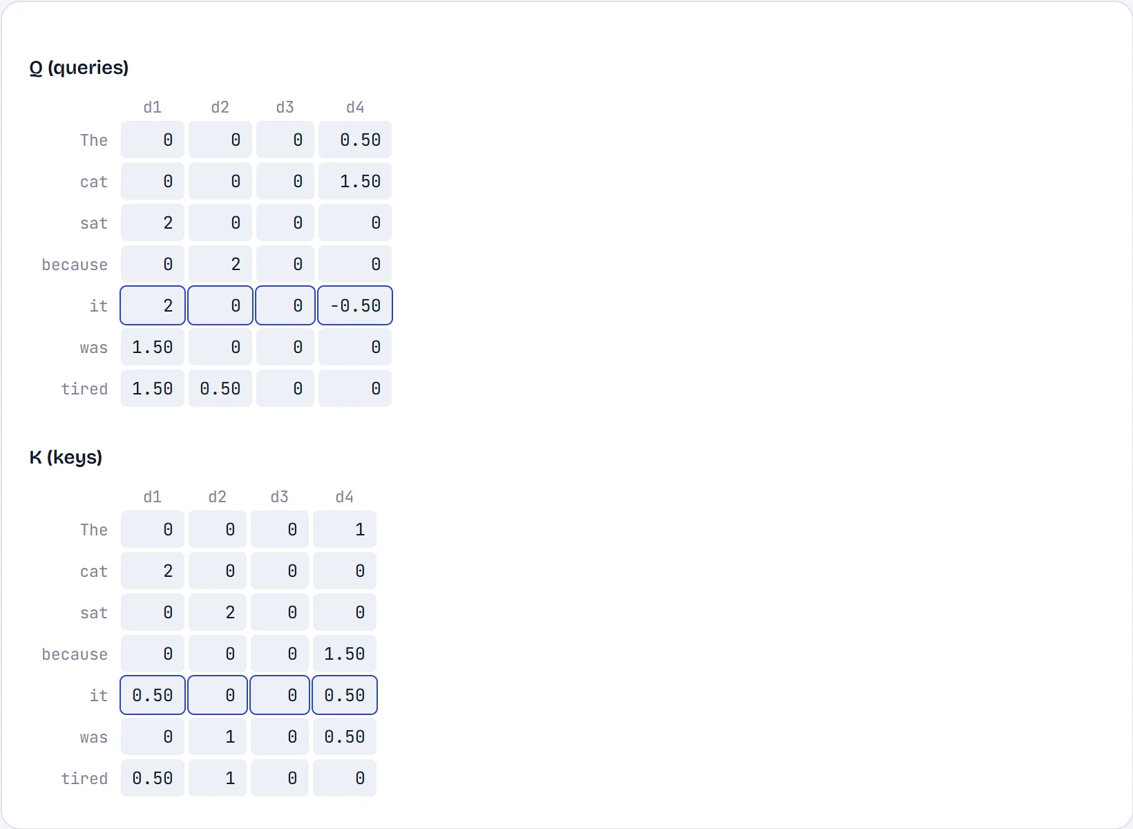
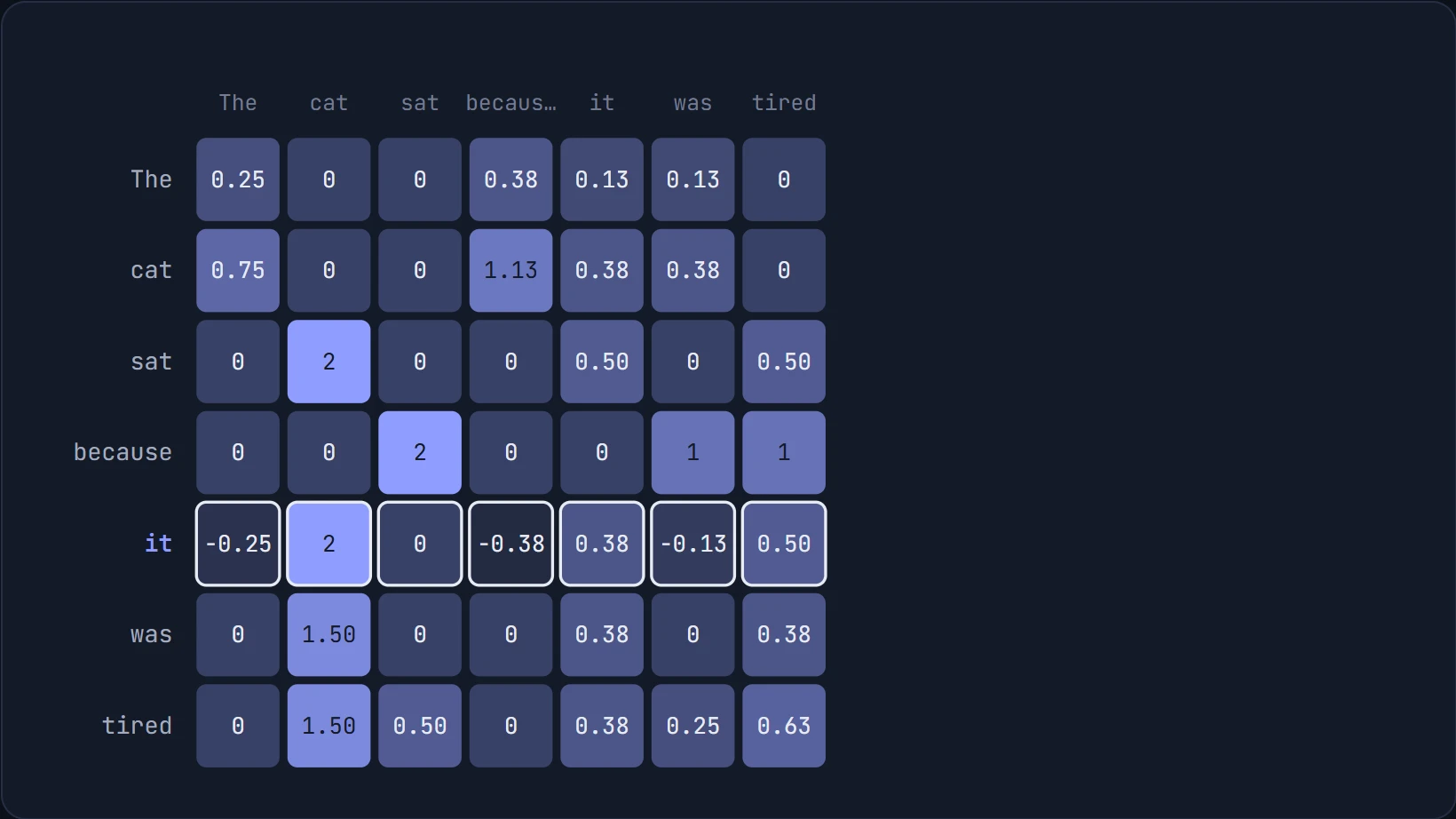
Step 1 of 6 1 · Project to Q and K Each token's embedding has already been multiplied by WQ and WK. Read the columns loosely as features: d1 ≈ “is an animal”, d2 ≈ “is an action”, d4 ≈ “is a little grammar word”. Look at “it”'s query: [2, 0, 0, −0.5]. It's hunting for animals and mildly avoiding grammar words. And “cat”'s key, [2, 0, 0, 0], advertises exactly that.
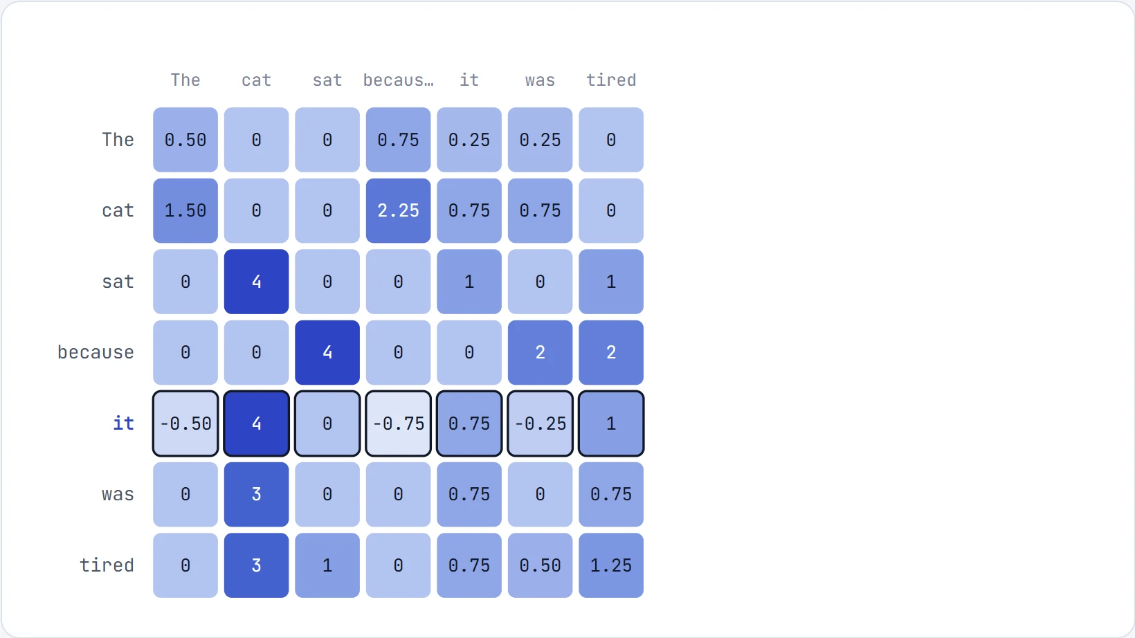
Step 2 of 6 2 · Score every pair: QKᵀ Every query is dotted with every key, giving a 7 × 7 grid. Row = who's asking, column = who's being asked. That's one matrix multiplication, which is why GPUs love this. Row “it”, column “cat”: q·k = 2·2 + 0·0 + 0·0 + -0.5·0 = 4.00. Notice the grid isn't symmetric. “it” → “cat” is 4.00, but “cat” → “it” is 0.75. Attention has a direction.
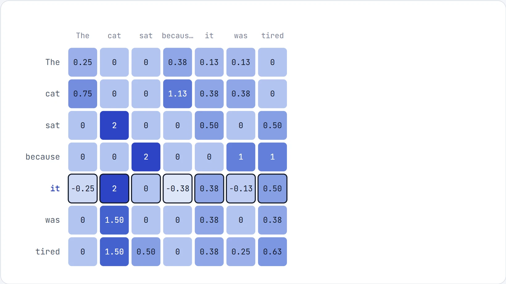
Step 3 of 6 3 · Scale by √dₖ Divide everything by √dₖ = √4 = 2. The ranking in each row doesn't change at all. Only the spread shrinks. With 4-number vectors this barely matters. With 128-number vectors it's the difference between learning and not learning. There's a whole section on why, coming up next.
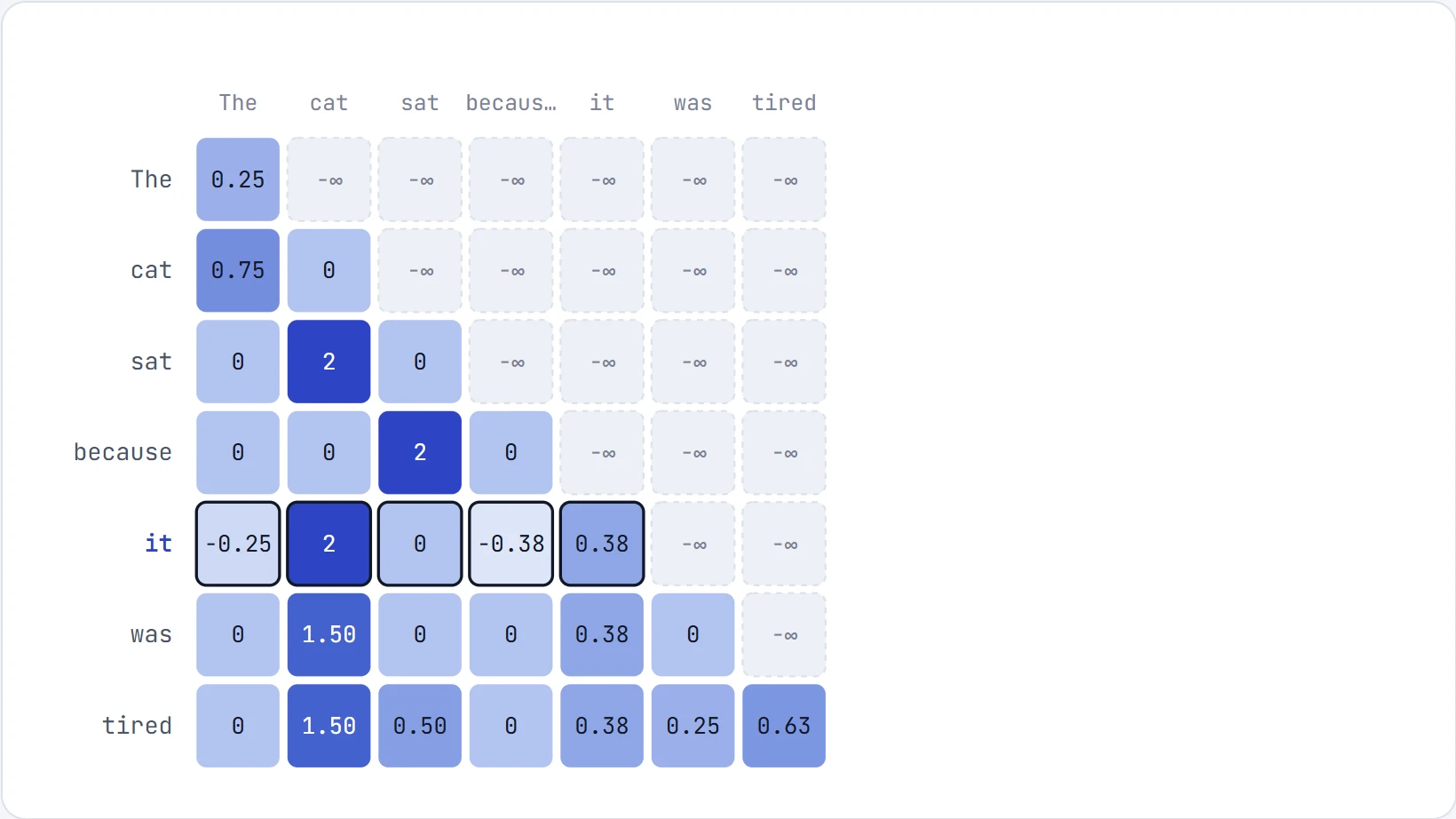
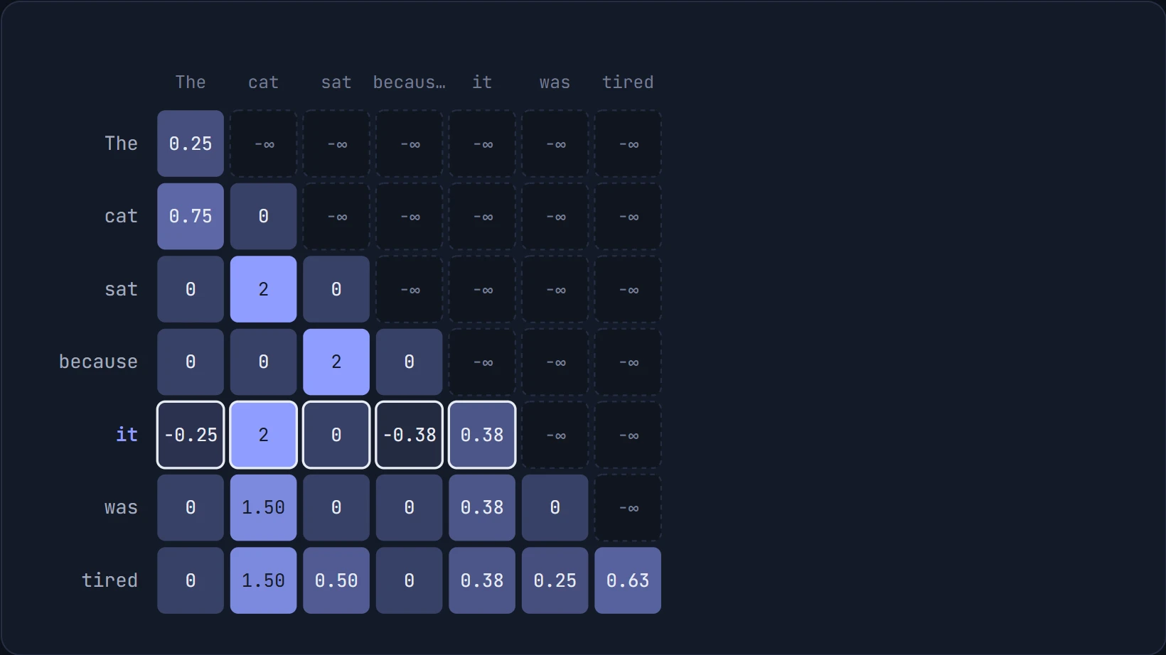
Step 4 of 6 4 · Mask the future Set every score above the diagonal to −∞. Row “it” may only see itself and the 4 words before it. Why −∞ and not 0? A score of 0 still gets a real share after softmax (e⁰ = 1). We need escore = 0, and only −∞ gives that.
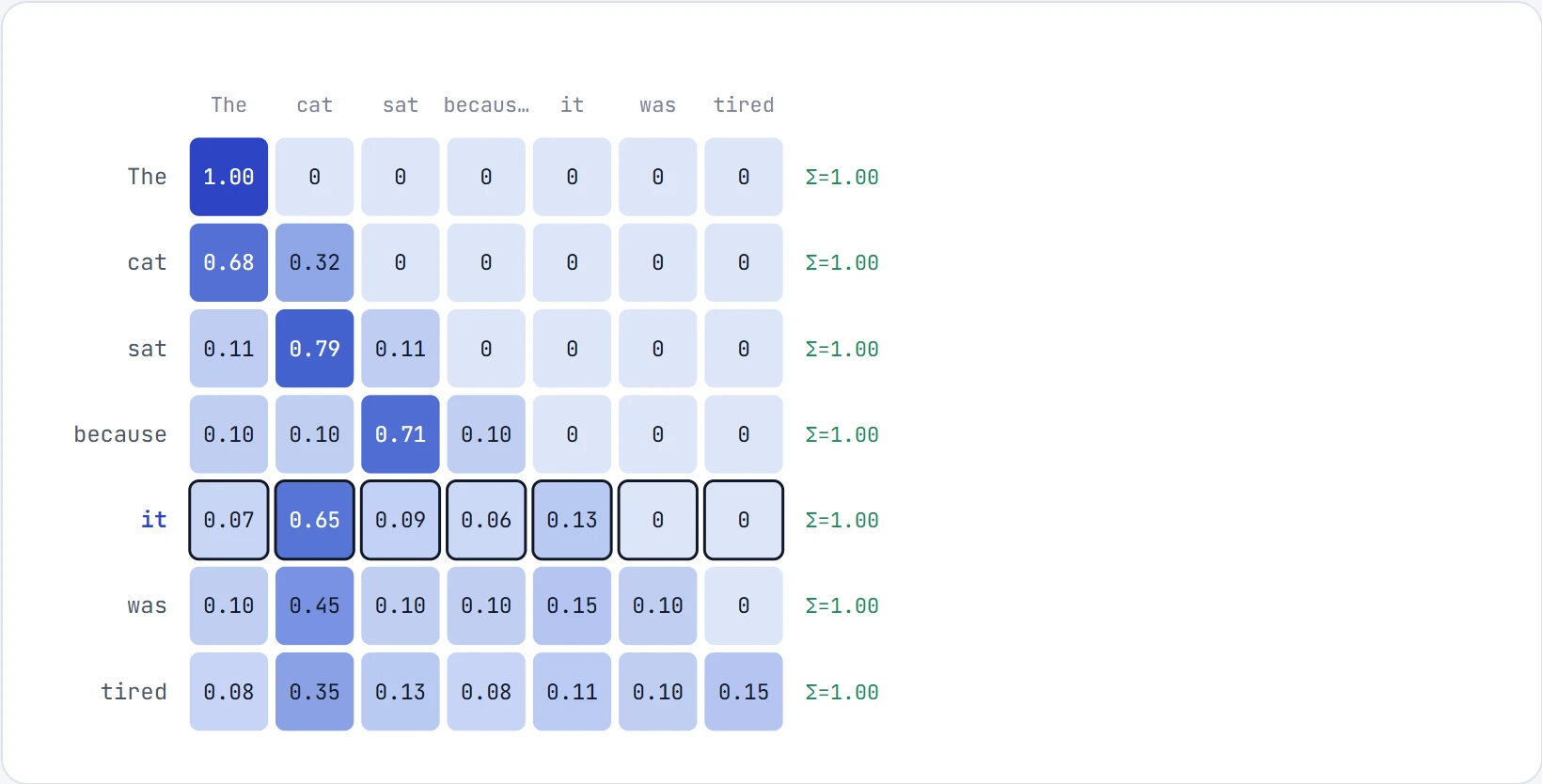
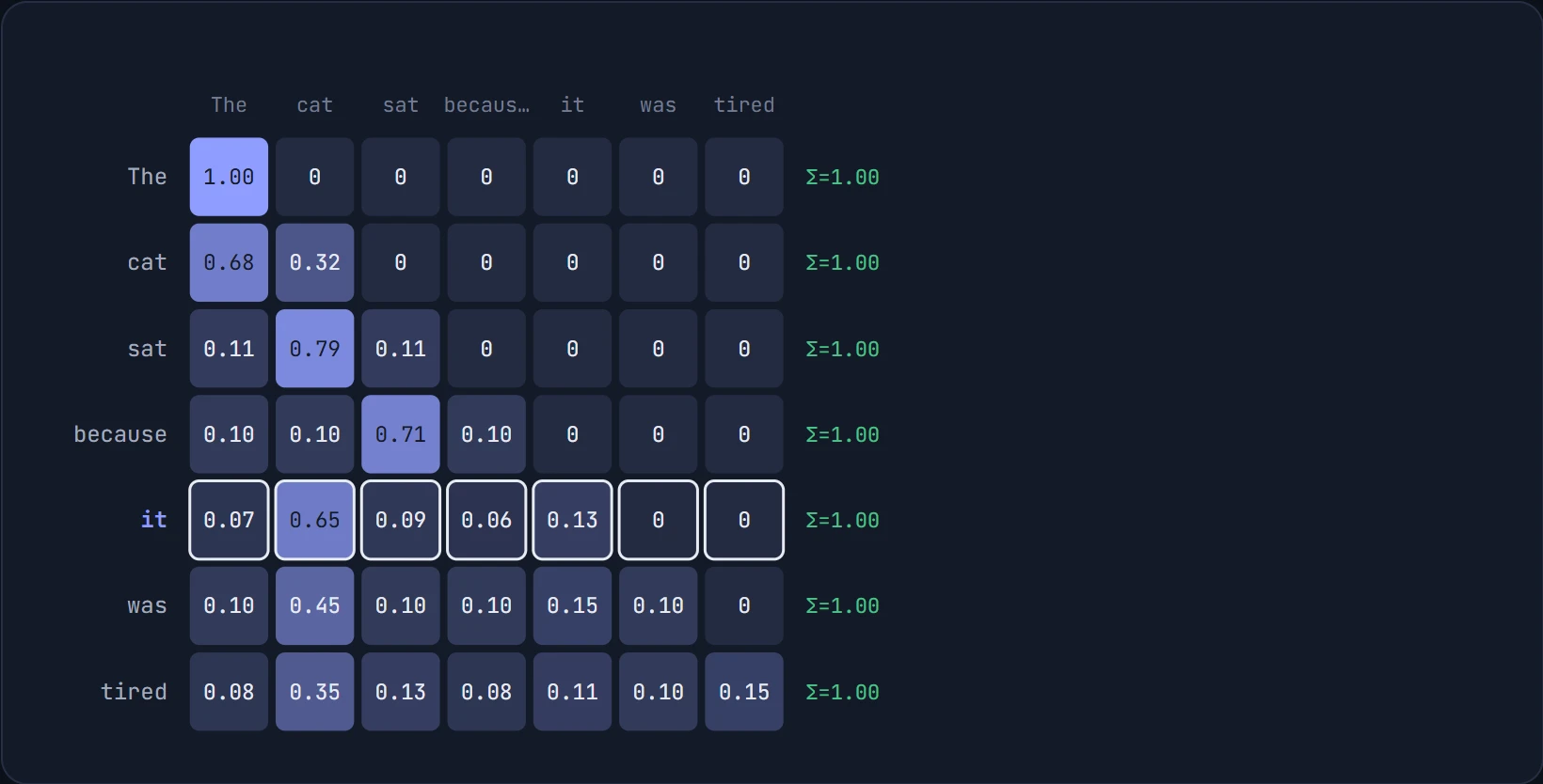
Step 5 of 6 5 · Softmax each row Each row becomes a set of weights that add up to 1 (the green Σ column). The masked cells get exactly 0. Row “it” gives 65% to “cat”. This grid is the attention pattern you saw at the top of the page.
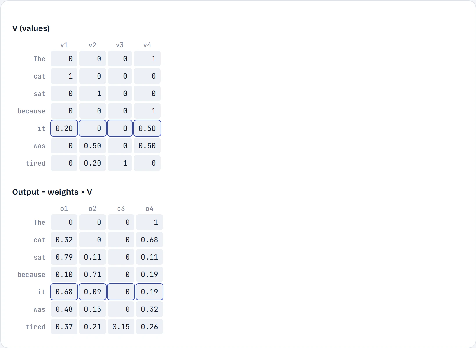
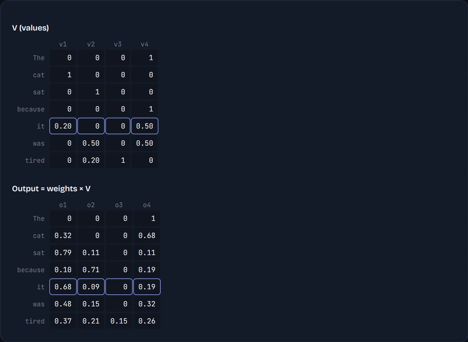
Step 6 of 6 6 · Mix the values Finally, each output row is a weighted average of the value rows, using that row's weights. Output for “it” ≈ 0.65·vcat + 0.13·vit + 0.09·vsat + … = [0.68, 0.09, 0.00, 0.19]. “it” now carries mostly “cat” information in its vector. The next layer no longer has to wonder what “it” refers to.
If you made it to step 6, you've computed attention by hand. Here's the formula from the 2017 paper that introduced the Transformer. Nothing in it should be new to you now:


Two parts of that formula look like housekeeping, and both turn out to matter a great deal. Let's take them one at a time.
The square root nobody puts on a poster
Our toy uses 4-number vectors. Real models use 64 or 128 per head.
Predict first. Take random query and key vectors whose numbers have mean 0 and spread (standard deviation) 1. If you double the vector length dₖ, how much bigger does a typical dot product q·k get?
- 2× bigger
- √2 ≈ 1.41× bigger
- 4× bigger
- No change
Answer. √2 bigger. A dot product is a sum of dₖ terms qᵢkᵢ. Each term has variance 1, and when you add independent random things, their variances add. So the variance of q·k is dₖ, and its typical size (the standard deviation) is √dₖ. Double dₖ and the typical size grows by √2. Dividing by √dₖ cancels that growth exactly, so the scores stay around size 1 at any width.
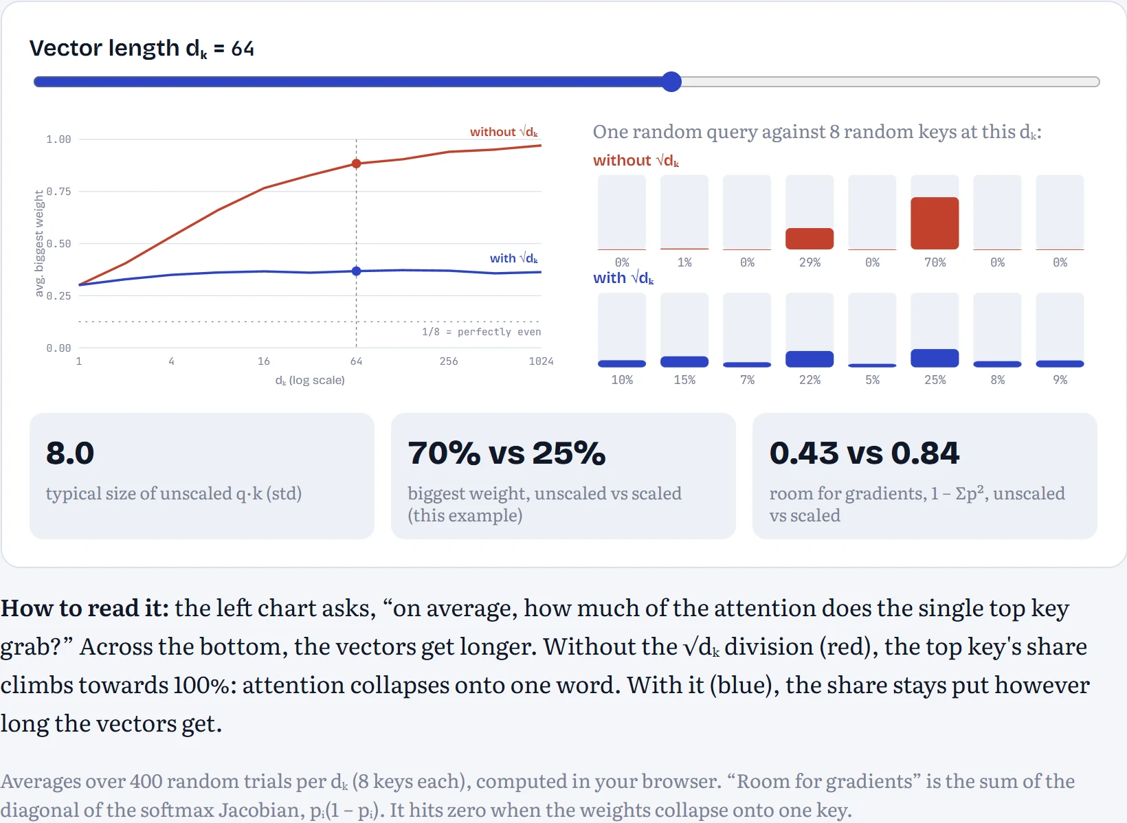
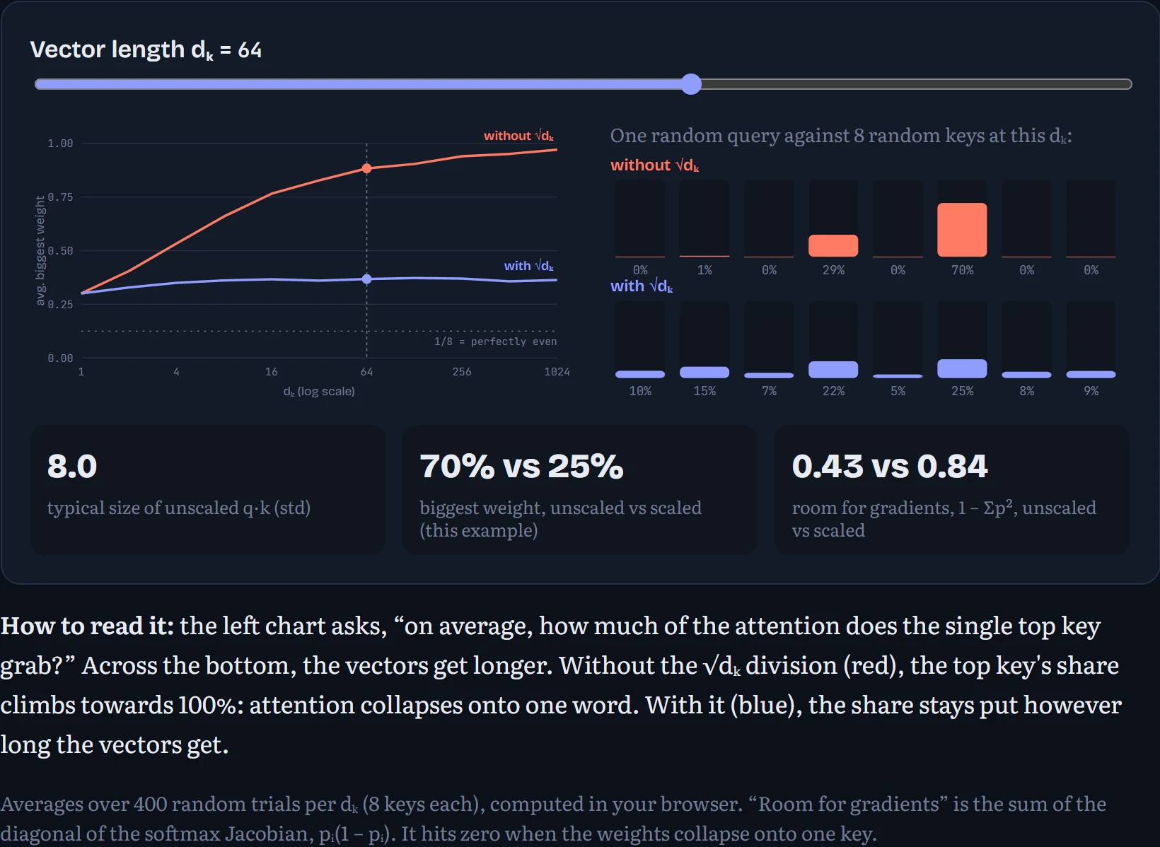
Here's why this matters for learning, not just tidiness. Without the division, scores at dₖ = 128 typically spread over ±11 and often reach ±20. Softmax of numbers that far apart is close to one-hot: one key routinely takes 90% or more and the rest get crumbs. The slope of softmax at that point is almost exactly zero (that's the “room for gradients” readout collapsing), so backpropagation sends back nearly nothing, and the attention pattern can't learn.
It's one division. It's also the difference between a model that learns and one that stares at a single token like it owes it money.
PRECISION NOTE. The exact √dₖ argument assumes unit-variance, independent components, which is roughly true at initialization. Trained weights don't keep that property, so in practice the scale mainly protects the early, fragile phase of training. Some modern models add extra normalization of q and k (“QK-norm”) for the same reason.
No peeking: the causal mask
A language model's job is to predict the next token. If “sat” could attend to “because”, it would be reading the answer key. So before softmax, we set every score where a token would look at a later token to −∞. Since e−∞ = 0, those positions get exactly zero weight, and the remaining weights still add up to 1.
That triangle buys something big. Because each row only sees its own past, one forward pass trains every position at once: seven predictions from one seven-token sentence, all computed in parallel. Your Chapter 8 RNN had to crawl through the sentence one step at a time. This is a large part of why Transformers train so efficiently on GPUs.
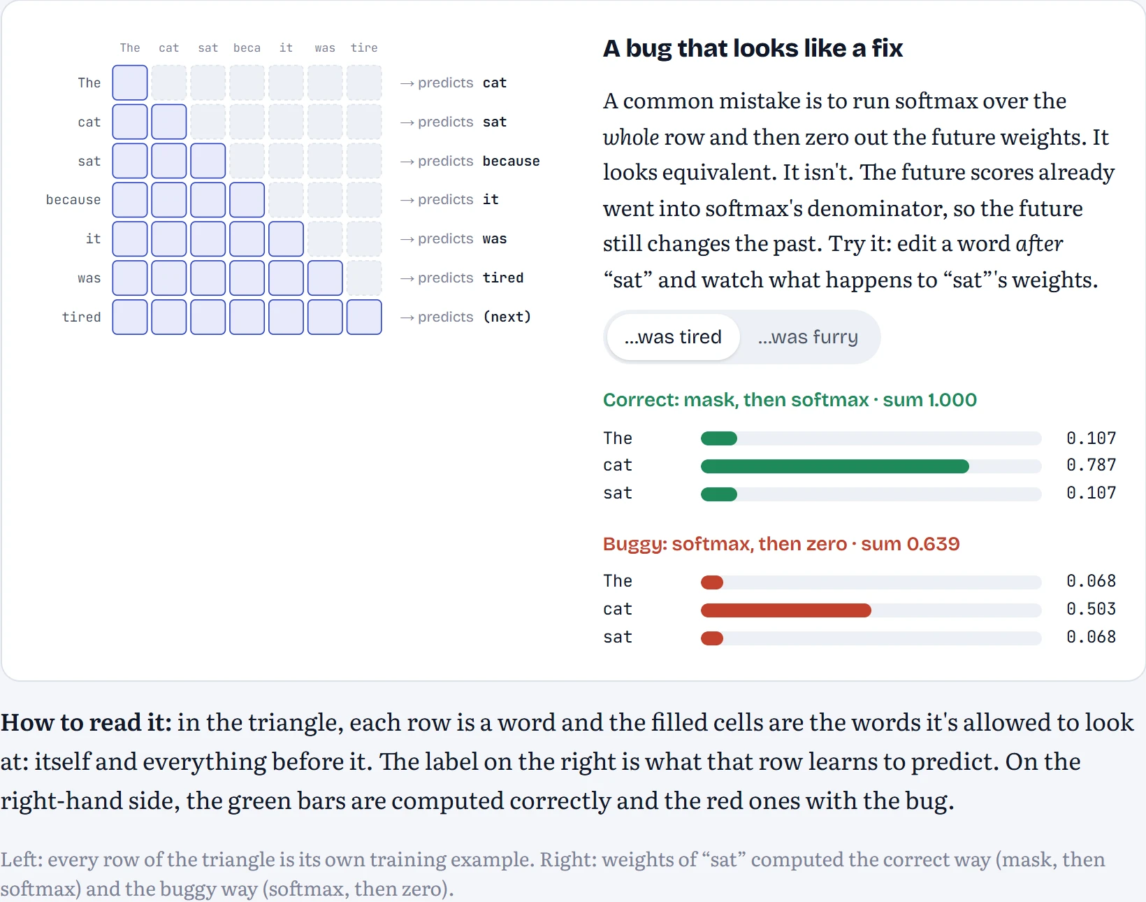
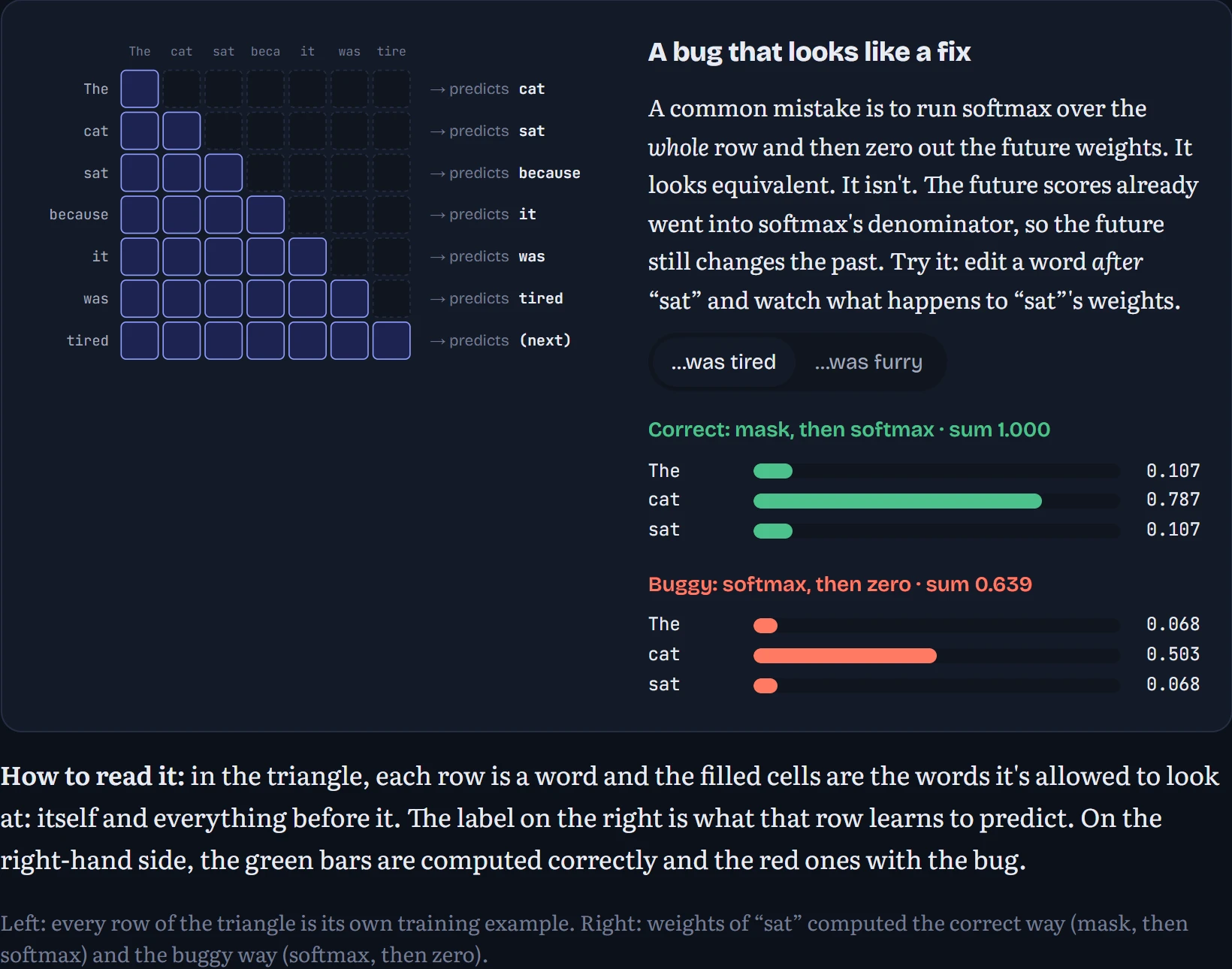
If your loss drops to nearly zero in the first hundred steps, congratulations: you haven't built AGI. You've built a model that reads the answer key. Check the mask first.
Many heads, one budget
One attention pattern per layer is restrictive. “It” wants to find its noun, but it might also want to know the word right before it, and whether the sentence is a question. One softmax can't point strongly in three directions at once, because the weights have to add up to 1.
The fix: slice the model's width into h independent pieces. If the model width is d_model = 512 and there are h = 8 heads, each head gets its own 64-number queries, keys and values and runs the exact computation you just stepped through. The eight outputs are glued back together and mixed by one more matrix, W_O.
Think of a panel of editors reading the same sentence, each with a different job: one checks grammar, one tracks who “it” refers to, one watches the punctuation. Each produces short notes, and the notes are combined at the end. Several narrow specialists see more than one generalist with the same total attention span. Below, three heads read our sentence; each grid has the same layout as the step-by-step grids above (rows look, columns are looked at), so you can compare their habits at a glance.
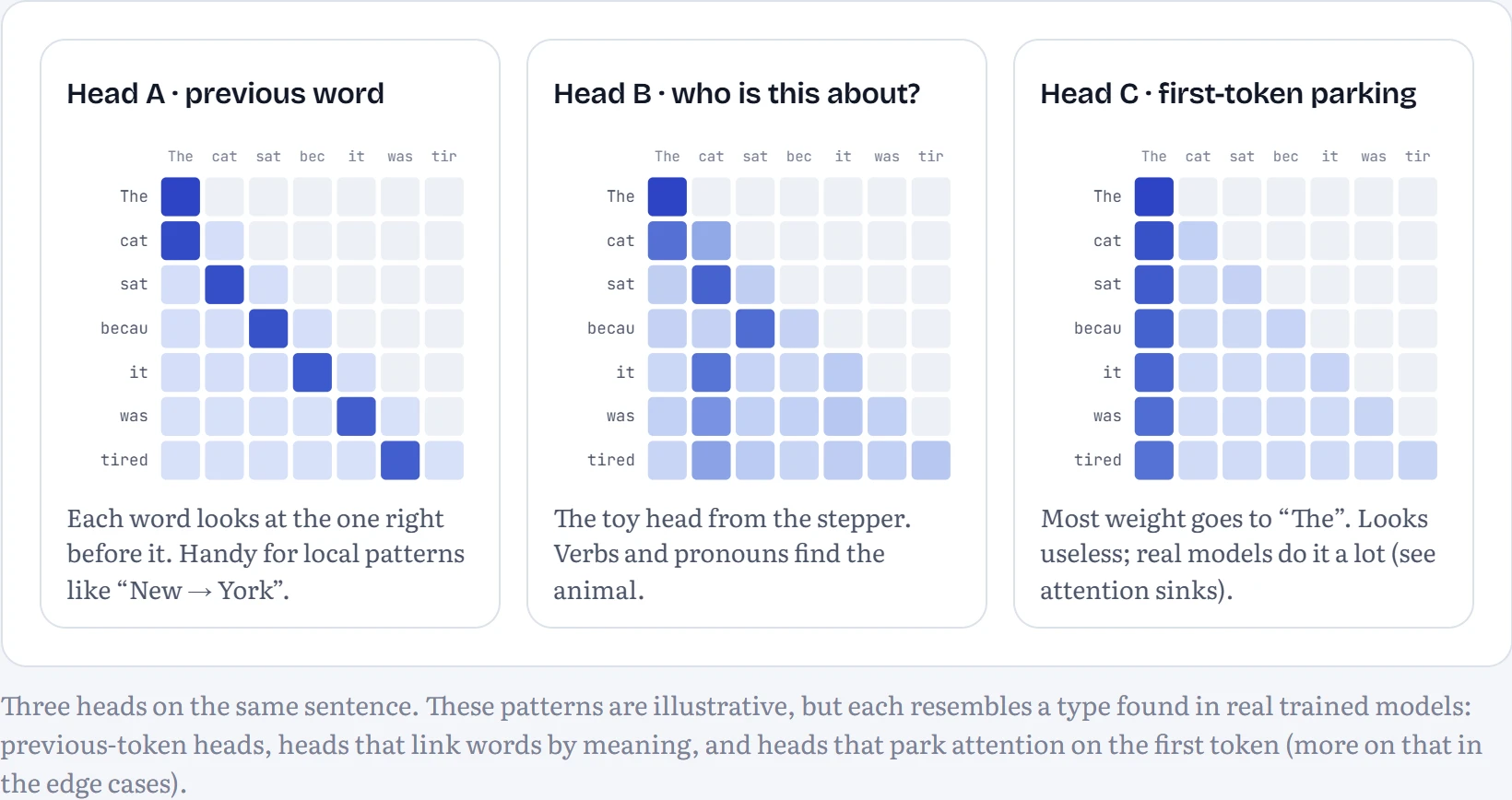
Here's the part people often get wrong: more heads doesn't mean more parameters. Each head is narrower, so the total stays the same.
Model width d_model
256
512
768
4096
Heads h
1
4
8
16
32
64 numbers per head (dₖ)
1.05M attention weights per layer
W_Q, W_K, W_V and W_O are each 512 × 512, whatever h is. Changing h only changes how those numbers are sliced: 8 heads of 64 numbers each.
Zoom out: where attention lives
The 2017 paper was called Attention Is All You Need. Bold title. Its biggest model also needed residual connections, layer normalization, an MLP after every attention layer, a carefully tuned learning-rate warmup, and eight GPUs for three and a half days. “Attention Is Most of What You Need, Plus Some Plumbing” just doesn't fit on a T-shirt.
Here's the whole stack, one zoom level at a time. In each panel, the highlighted part is what the next panel opens up.
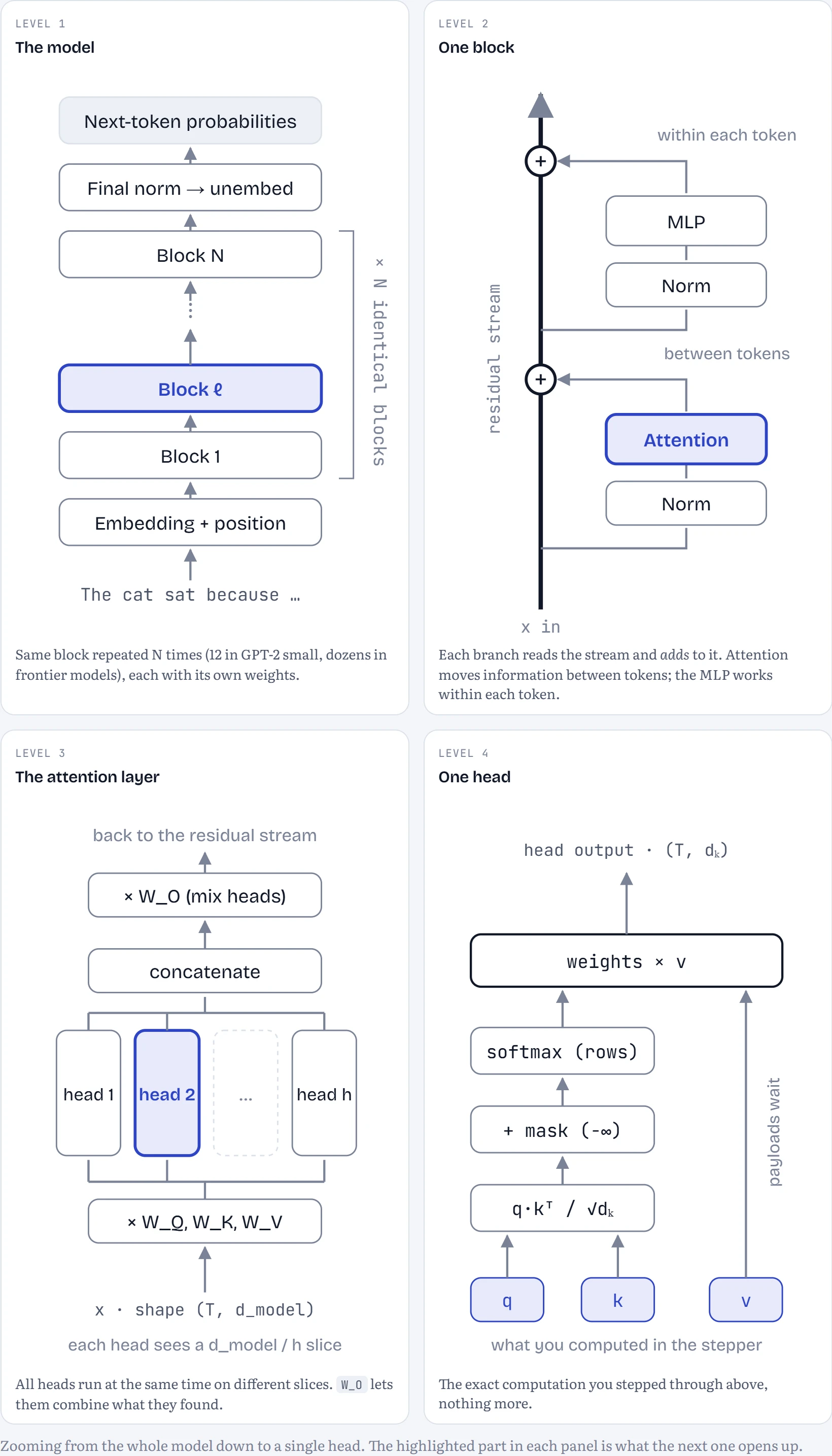
The residual stream is the real backbone
Look at Level 2 again. The thick line going straight up is the residual stream: each token's vector, passed from block to block. Sublayers never replace it. They read a normalized copy and add their result back. You met residual connections in Chapter 5 as a trick to keep gradients flowing through deep networks. Here they become the architecture's main communication channel. Every head and every MLP in every layer reads from the same shared stream and writes into it.
That's also where the “new information” comes from that attention can't make on its own. Attention only blends existing vectors. The MLP that follows applies a non-linear function to each token separately, so it can compute genuinely new features from what attention gathered. Roughly: attention decides what to bring over, the MLP decides what to make of it.
OPEN RESEARCH. Interpretability work suggests that much of a model's factual recall happens in the MLP layers, while attention heads route information. That's a useful working picture backed by real experiments, not a settled law. Chapter 15 shows you how to test claims like this on your own model.
Continue the lesson
The whole lesson, with its drawings and its questions. 4 more sections after the ones above.