
Inductive biases: convolutions, residual connections, GRUs and backpropagation through time
An architecture bakes assumptions about the data into the network, called inductive biases. Convolutions assume nearby pixels matter together and a pattern means the same thing anywhere. Recurrence keeps a memory that updates token by token. When an assumption is wrong for your data, the architecture fights you.
What this page answers
What is an inductive bias?
An assumption about the data built into a network's architecture, such as locality and translation equivariance for images. It saves the network from learning those facts separately at every position. Read it in “Built-in assumptions”
Why do RNNs forget long sequences?
An unrolled RNN is a very deep network: the gradient reaching k steps back has been multiplied by k Jacobians. If they shrink the signal, the influence of anything far back fades exponentially. Read it in “Backprop through time, and the vanishing gradient”
Built-in assumptions
The MLP from Chapter 5 treats a 28 × 28 image as a list of 784 unrelated numbers. Its first layer connects every pixel to every hidden unit, so it has no idea that pixel 1 is next to pixel 2: if you shuffled the pixels in the same fixed way for every image, before training, it would learn just as well. That sounds like flexibility. It's actually a handicap, because the network must learn from examples what every human knows from birth, and it must learn it separately for every position. A stroke in the top-left corner and the same stroke in the bottom-right corner are, to an MLP, completely different patterns.
It also scales terribly. A 1,000 × 1,000 colour photo has 3 million inputs; one fully connected layer with 1,000 units would need 3 billion weights. Architecture lets us bake in assumptions, called inductive biases, that are true of the data: for images, locality (nearby pixels matter together) and translation equivariance (a pattern means the same thing wherever it appears). The price is that if an assumption is wrong for your data, the architecture fights you. You can test that directly.
Predict first. I trained an MLP and a small CNN on MNIST twice each: once on normal digits, and once on digits whose 784 pixels were scrambled by one fixed random permutation (the same scramble for every image, train and test). Which model is hurt by the scrambling?
- Both, equally
- The MLP
- The CNN
Answer. The CNN. Scrambling cost it 3.7 percentage points (98.65% → 94.93%), while the MLP barely noticed (97.05% → 96.77%, a difference the size of a different random seed). The MLP never assumed anything about which pixels are neighbours, so a fixed reordering is just a relabelling. The CNN's whole design rests on neighbours mattering together, and after scrambling, its 5 × 5 filters look at 25 pixels from random places all over the image. It still learns something, because a fixed permutation is consistent, but its advantage is gone.
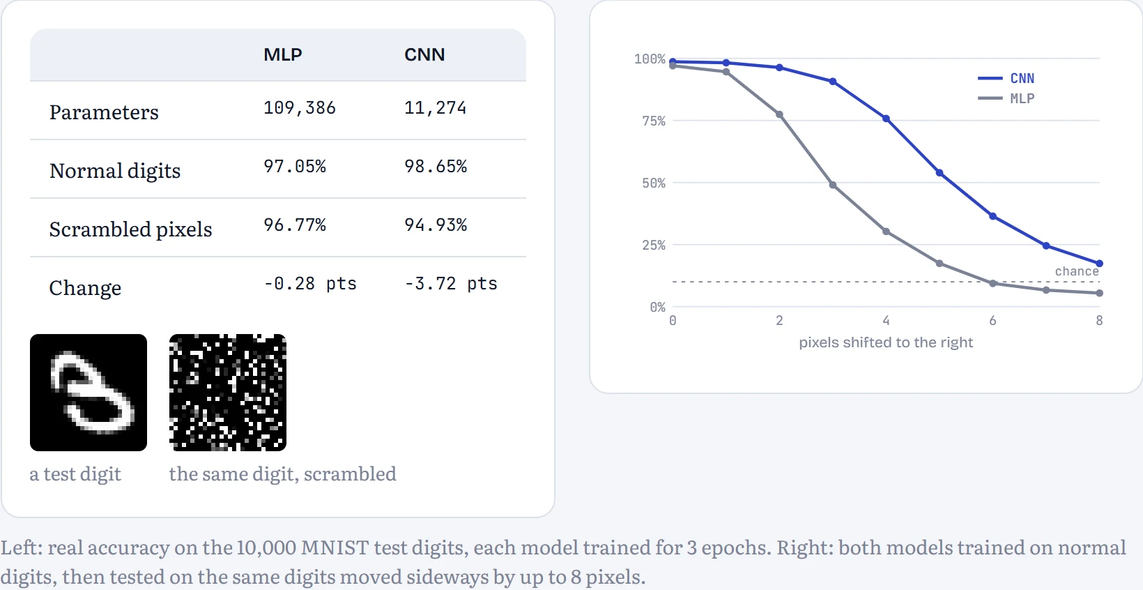
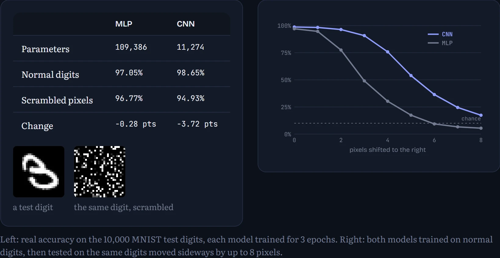
How to read the table and chart: the table compares accuracy with normal and scrambled pixels; the chart shows what happens when a digit is drawn a little off-centre. The MLP has never seen a digit moved by more than a pixel or two (MNIST digits are centred), and at a 3-pixel shift it's down to 49%. The CNN, with a tenth of the parameters, still gets 91%: its filters detect a stroke wherever it is, and max-pooling forgives small moves. Its robustness isn't unlimited, though. The final fully connected layer still cares where features ended up, so by 6 pixels it falls below half too. That's the honest version of the textbook claim: convolution makes features equivariant (move the input and the feature map moves with it), and pooling buys a little invariance; full invariance needs more pooling or data augmentation.
So an inductive bias is a bet. When it matches the data, as locality does for images, you get better accuracy from fewer parameters and less data. When it doesn't, as with scrambled pixels, it actively hurts.
Convolution: one small filter, slid everywhere
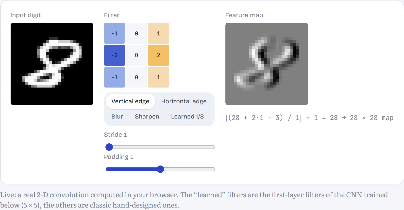
A convolutional layer replaces “every pixel connects to every unit” with a small grid of weights, a filter (or kernel), say 3 × 3, that is slid across the whole image. At each position it multiplies its 9 weights by the 9 pixels underneath, adds them up, and writes one number into an output image called a feature map. The same 9 weights are used at every position, which is parameter sharing: a filter that detects a vertical edge detects it everywhere. A layer has many filters, each producing its own map, and the next layer's filters look across all of those maps at once.
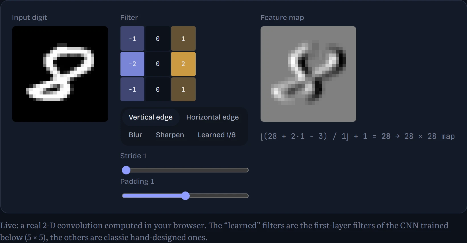
Two knobs control the output size. Stride is how far the filter moves each step (stride 2 halves the size); padding adds a border of zeros so the filter can sit on edge pixels. For an input of width n, filter size k, padding p and stride s, the output width is ⌊(n + 2p − k) / s⌋ + 1. In the figure: a filter with its stride and padding; the right panel shows the feature map, with bright for strongly positive responses and dark for negative.
Stack a few layers and something useful happens. A unit in the first layer sees a 5 × 5 patch; after a pooling step (which shrinks each map by keeping the largest value in every 2 × 2 block) and another 5 × 5 filter, a unit in the second layer sees a 14 × 14 region of the original image. That growing receptive field lets early layers detect edges, middle layers combine edges into strokes and corners, and late layers combine those into whole digits or, in big networks, faces and wheels.
A CNN, live
This is the CNN from the scrambling experiment: two convolution layers (8 filters, then 16, each 5 × 5), each followed by a ReLU and 2 × 2 max-pooling, then one fully connected layer to the 10 digits. 11,274 parameters and 98.65% test accuracy. In the lesson it runs in your browser, with every feature map updating as you draw.
Each first-layer filter responds to a drawing in its own way. Some light up along vertical strokes, others along horizontal or diagonal ones, and some on the background around strokes. The second layer, at half the resolution, responds to combinations: corners, loops, stroke ends.
Going deeper: the residual trick
From LeNet (LeCun and colleagues, 1998: a few layers, handwritten digits) to AlexNet (Krizhevsky and colleagues, 2012: eight layers, ImageNet, the start of the deep learning boom) to VGG (19 layers), progress came largely from depth. Then it stalled: beyond about 20 layers, deeper networks trained worse, even on their training data. Chapter 5 showed why: every layer multiplies the backward signal, so gradients shrink or explode over many layers. ResNet (He and colleagues, 2015) fixed it with one line: instead of h = F(h), compute h = h + F(h). Each block only adds a correction to its input, and the “+ h” path carries both the signal forward and the gradient backward untouched, however deep the stack. ResNets trained with over 150 layers.
Demonstrating this took me four attempts, which is a lesson in itself. With convolution layers and batch normalization on MNIST, plain stacks of up to 32 layers trained fine in a short run and residual connections added nothing: normalization had already solved most of the problem at that depth (Chapter 9 shows how it keeps signals in range). Without normalization, my first residual stack blew up instead, because the corrections from 20 blocks piled on top of each other. So the clean test strips everything else away: a stack of fully connected layers with no normalization. The plain version is h = relu(W·h + b), with the best initialization a plain ReLU stack can get. The residual version uses blocks h = h + W₂·relu(W₁·h) whose W₂ starts at zero, so every block begins as “do nothing” and learns a correction from there. Both are 128 units wide and get the same 600 training steps. How to read the charts: left, test accuracy against the number of layers (log scale); right, training loss during the run for the two deepest settings.
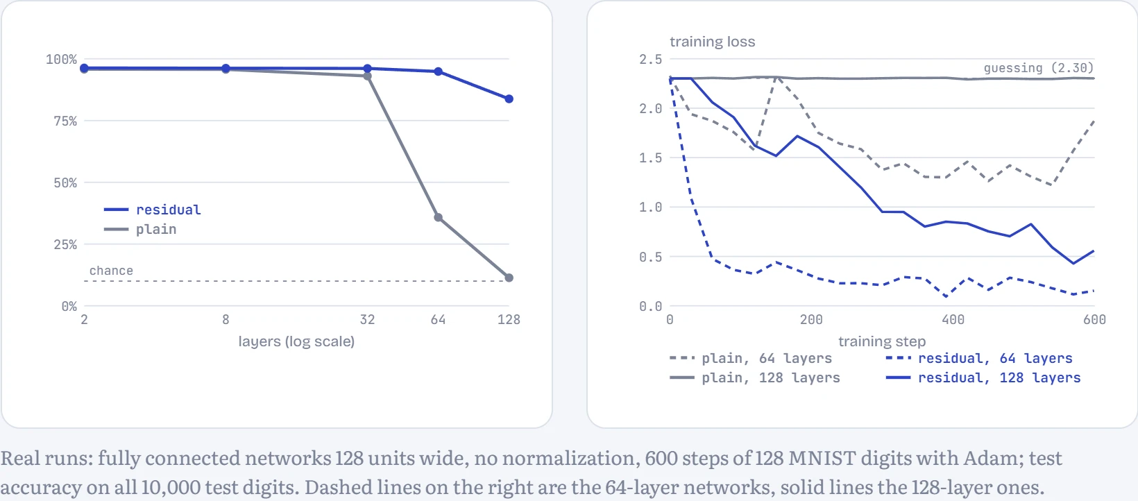
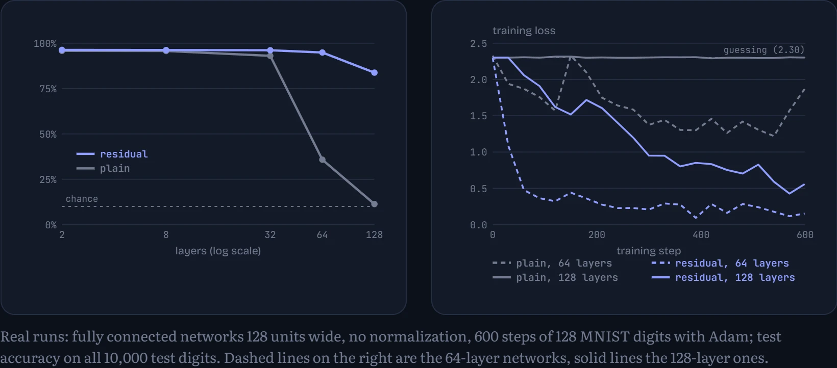
At 2 and 8 layers the two are neck and neck (95.8% against 96.3% at 2). Then the plain stack falls apart: 93.0% at 32 layers, 35.8% at 64, and at 128 layers 11.3%, which is guessing. The right chart shows it never got started: its loss sits at 2.30, the loss of a uniform guess over 10 digits, for the whole run. The residual stack keeps learning at every depth: 94.9% at 64 layers and 83.8% at 128. It does get somewhat worse at extreme depth in a short run, since there is more to train, but it's learning the whole time.
Why the difference? At the start, every residual block is the identity, so a 128-layer residual network is a one-layer network, and the gradient reaching its first layer is exactly the same at every depth (1.69 at 2 layers, 1.69 at 128). Each block then learns to add a little, and the “+ h” path keeps carrying the signal and the gradient straight through, however many blocks there are. The plain stack has to push everything through 128 matrix multiplications and ReLUs, each one a chance to distort the signal, and small distortions compound. This is the idea every Transformer is built on: each attention or MLP block in Chapter 9 adds its output to a residual stream instead of replacing it.
Convolutions aren't just for images. A 1-D convolution slides a filter along a sequence instead of across a grid: over audio samples, over the frames of a spectrogram, or over word embeddings. The speech recognizer in Chapter 14 starts with two of them, each looking at five 10-millisecond frames at a time, before handing over to a recurrent layer. That hand-over is where the next part of the story begins.
Recurrence: a memory that updates
Your mini_lm from Chapter 7 read a fixed window of 16 characters. Anything earlier was invisible, and making the window bigger means more weights. A recurrent neural network reads one character at a time and carries a hidden state, a vector that summarizes everything read so far. At each step it combines the new input with the old state: ht = tanh(Wx·xt + Wh·ht−1 + b). The same weights are used at every step (parameter sharing again, this time across time), so it can, in principle, read sequences of any length.
The plain version has trouble remembering for long, for reasons we'll measure in a moment. The fix was gates: learned switches between 0 and 1 that decide how much of the old state to keep. The LSTM (Hochreiter and Schmidhuber, 1997) keeps a separate memory cell with forget, input and output gates; the GRU (Cho and colleagues, 2014) simplifies this to an update gate z and a reset gate r: ht = (1 − z) ⊙ candidate + z ⊙ ht−1. When z is near 1, the old state passes through almost untouched, the same idea as the residual connection, applied across time instead of depth.
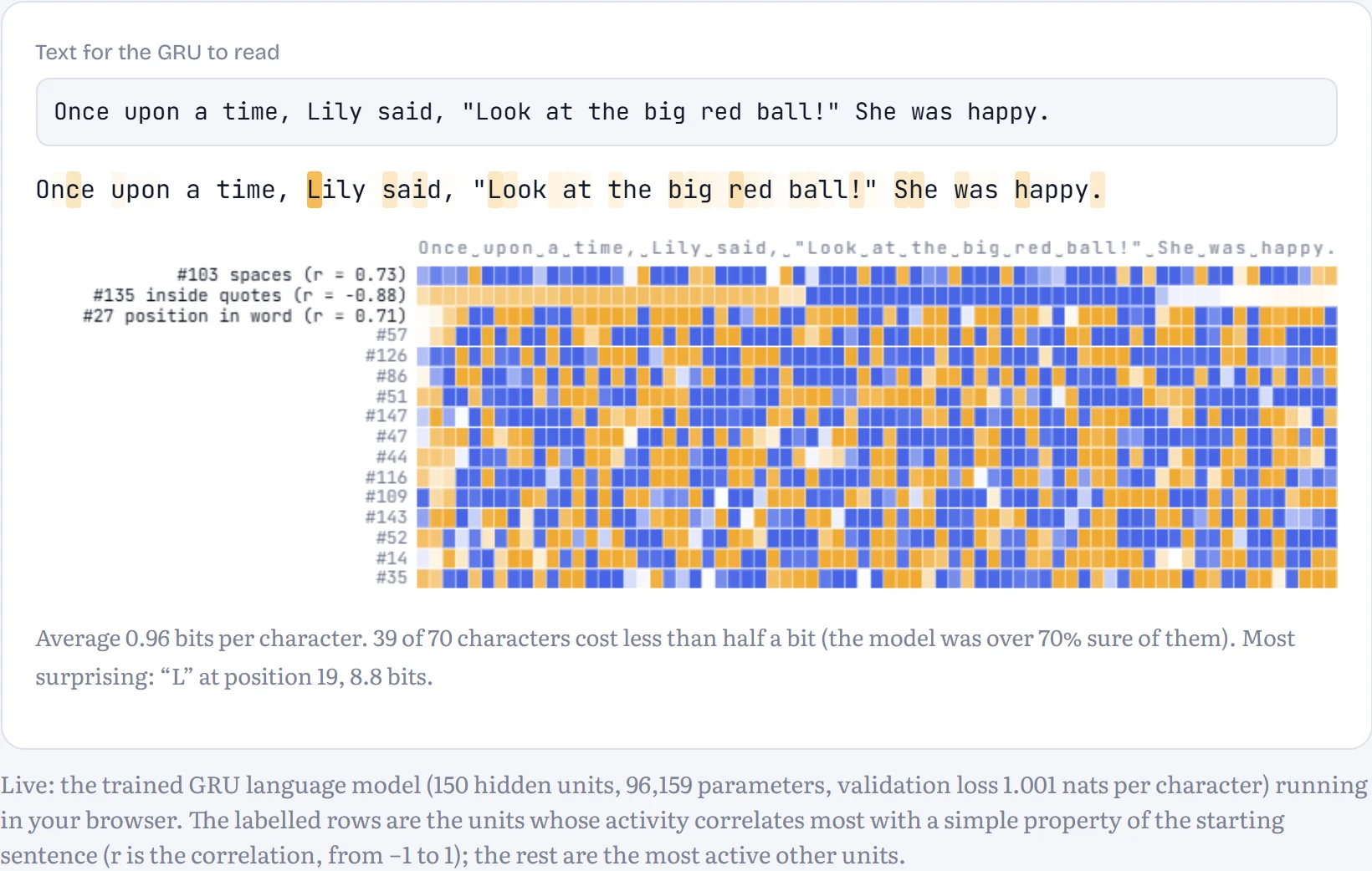
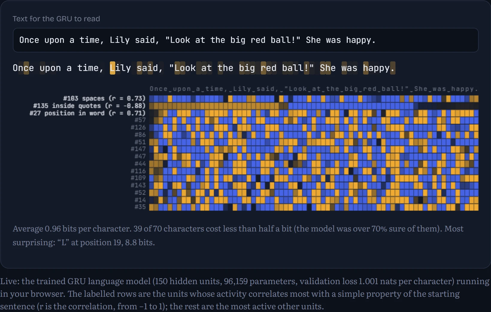
Here's a GRU language model I trained on stories, reading your text live. How to read it: each character is shaded by how surprised the model was to see it (stronger shading = more surprising, measured as −log₂ of the probability it predicted); below, each row of the heat map is one of 16 hidden units over time, blue for negative and amber for positive. Nobody told any unit what to track, yet some line up with spaces, quotes or position within a word: those are labelled.
Which recurrent cell is best? I trained all three as character language models with about the same number of parameters, on the same data, for the same number of steps. How to read the chart: loss on held-out stories (lower is better) as training proceeds.
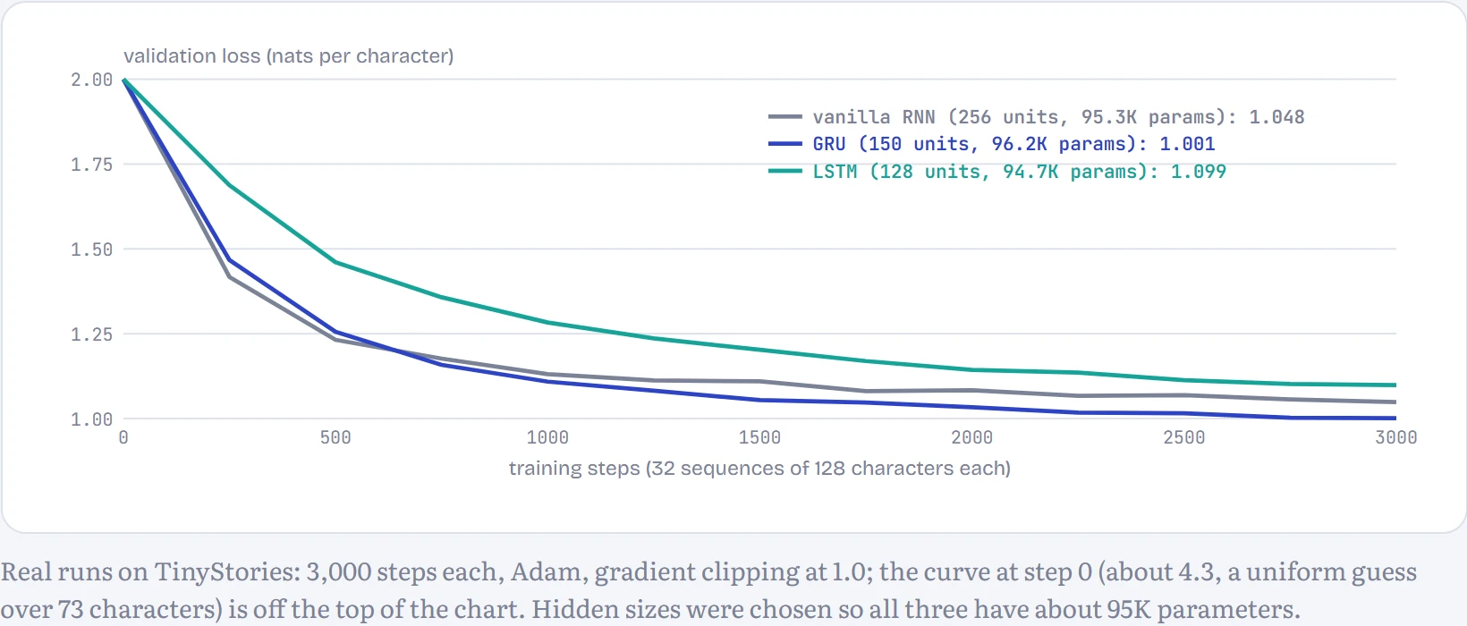
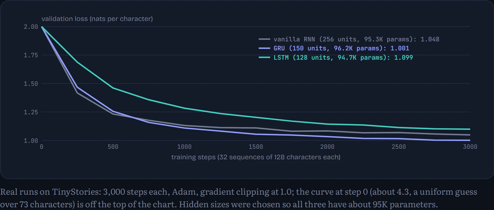
The GRU finished best (1.001), then the vanilla RNN (1.048) and the LSTM (1.099). The spread is small: about 0.14 bits per character between best and worst. Two things explain why gates matter less than you might expect here. At equal parameter count the vanilla RNN gets 256 hidden units against the LSTM's 128, because each gate costs another set of weights. And predicting the next character in a children's story mostly depends on the last few characters: finishing “Onc” or “happ” needs no long memory at all. Next-character loss is a blunt instrument for long-range memory, so let's measure memory directly.
Backprop through time, and the vanishing gradient
To train an RNN, unroll it: one copy of the network per time step, all sharing weights, and run ordinary backprop through the whole chain. That's backpropagation through time. The trouble is the same as in a very deep network, because an unrolled RNN is a very deep network: the gradient reaching step t − k has been multiplied by k Jacobians on the way back. If they shrink the signal, the influence of anything far back fades exponentially and the network can't learn long-range dependencies. In practice the unroll is also cut off after a fixed number of steps (truncated BPTT), here 128 characters.
We can measure the fading directly. How to read the chart: I fed each trained model 200 characters and computed how strongly the loss at the last character depends on the hidden state k steps earlier (the size of the gradient), on a log scale. A flat line means distant steps still matter; a steep fall means they're forgotten.
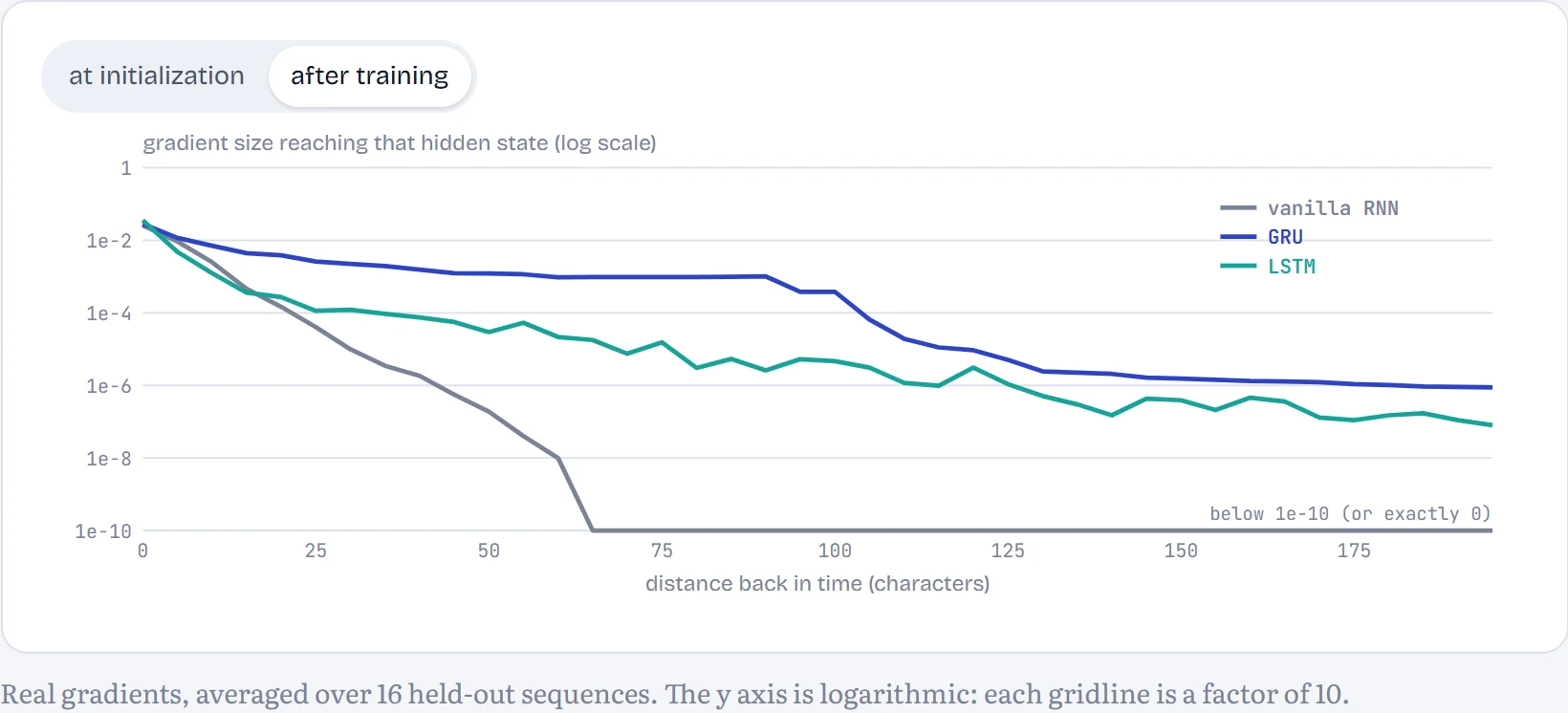
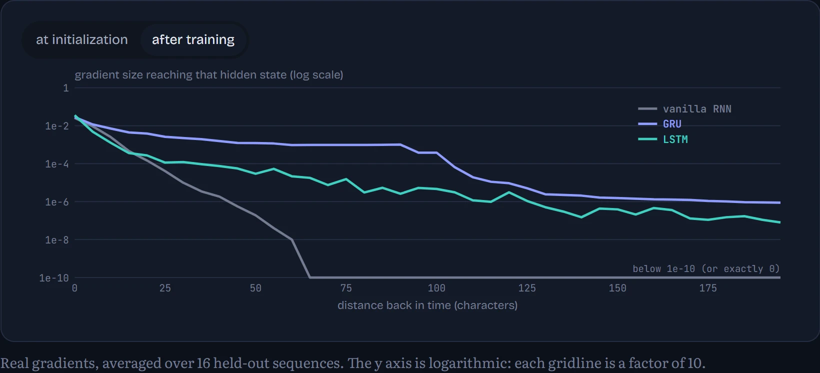
In the trained vanilla RNN, the gradient 50 characters back is 7 × 10⁻⁶ of its size at the last character; 25 characters back it's already 2 × 10⁻³. Whatever happened 50 characters ago, the training signal can't reach it, so the network has no way to learn to use it. The gated cells fade too, but far more slowly: 50 characters back the GRU still keeps 4 × 10⁻², and 100 characters back 1 × 10⁻². That's the update gate at work: when z is close to 1 for a unit, the state passes through nearly unchanged and so does the gradient, the same trick as the residual “+ h”.
Switch to at initialization to see the before picture: before any training, the gated cells already pass more gradient than the plain RNN. Training then taught the GRU to keep some gates nearly shut, building long-lived memory units.
The opposite failure, exploding gradients, makes training jump wildly; the standard fix, used in every run on this page, is gradient clipping: if the gradient's overall size exceeds a limit, scale it down before the update.
Continue the lesson
The whole lesson, with its drawings and its questions. 6 more sections after the ones above.