
Supervised learning: least squares, logistic regression and softmax classifiers
Every machine learning system is data, a model with adjustable parameters, a loss that says how wrong it is, and an optimizer that lowers the loss. This lesson fits a line two ways, then turns the same recipe into logistic regression for yes or no and softmax regression for ten digits.
What this page answers
What are the parts of a machine learning model?
Data, a model with adjustable parameters, a loss that measures how wrong it is, and an optimizer that changes the parameters so the loss goes down. Training is running the optimizer until the loss stops improving. Read it in “The recipe”
What is self-supervised learning?
Learning where the labels are cut out of the data itself. A language model learns this way: every position in a text is an example whose label is the character that comes next, so no human labels anything. Read it in “The recipe”
The recipe
Every machine learning system in this course, from a straight line through a scatter of points to a language model with billions of weights, is built from the same four ingredients. Data: examples of the thing you want. A model: a function with adjustable numbers inside, called parameters (or weights). A loss: a single number that says how wrong the model is on the data. An optimizer: a rule for changing the parameters so the loss goes down. Training is just running the optimizer, over and over, until the loss stops improving. Everything else is detail, though some of the detail is important.
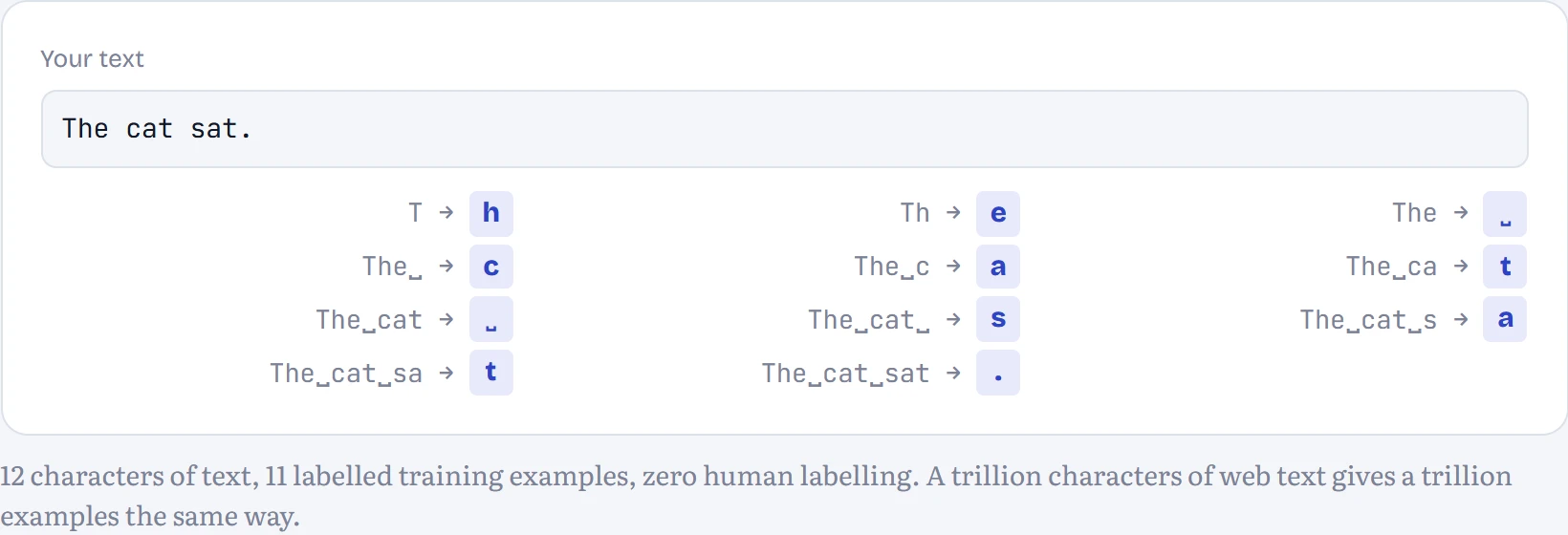
What changes between kinds of machine learning is where the right answers come from. In supervised learning, every example comes with a label someone provided: this scan shows a tumour, this email is spam. In unsupervised learning there are no labels, and the job is to find structure, such as groups of similar customers. In reinforcement learning there are no right answers at all, only rewards after actions, like points in a game. And in self-supervised learning, the labels are cut out of the data itself. That last one is how language models learn: every position in a text is an example whose label is simply the character that comes next. No human labels anything, which is why you can train on the whole internet.
In the figure: Each row below is one training example the text generated for free: the characters so far, and the label the model must learn to predict.
One more distinction you'll use constantly. Parameters are learned from data. Hyperparameters are choices you make before training starts: how big the model is, how big each step is (the learning rate), how long to train. The optimizer never touches them; you pick them by trying a few settings and comparing the results on data the model hasn't trained on. That last clause turns out to be the most important rule in the chapter.
Predict first. Your Chapter 1 bigram model, rebuilt as a neural network: the current character goes in, a probability for each possible next character comes out, with one weight for every (current, next) pair. Our stories use 69 different characters. How many parameters does it have?
- 69
- 69 × 69 = 4,761
- 2 × 69 = 138
Answer. 4,761, exactly the number of cells in the count table. It's the same model in a different costume: instead of counting, it will learn each of those numbers by gradient descent. The lab at the end of this page trains it and checks that it arrives at the same probabilities the counts give.
Fitting a line through real patients
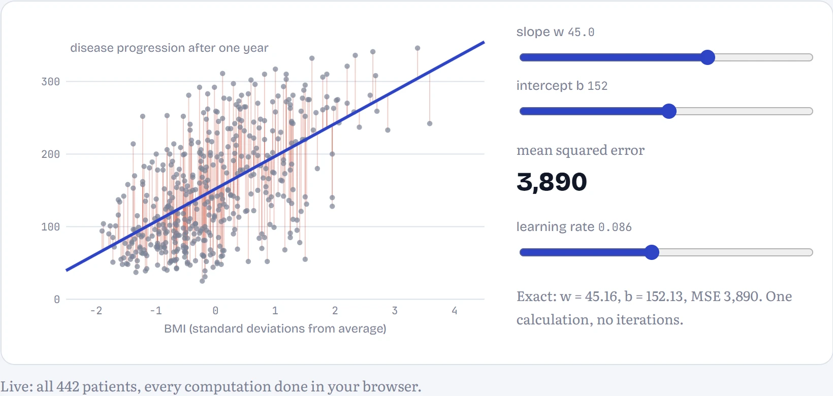
Here's a real dataset, one that comes bundled with scikit-learn (the standard Python machine learning library): 442 diabetes patients, each with ten measurements taken at the start of a study, and a number describing how far their disease had progressed a year later. Bigger is worse. Let's start with one measurement, body mass index (BMI), and the simplest model there is: a straight line, prediction = w × BMI + b. Two parameters: the slope w and the intercept b.
To score a line, measure how far each prediction misses the real value, square it (so misses above and below both count, and big misses count a lot more), and average over all patients. That's the mean squared error, MSE. In the figure: a line fitted by hand, with its MSE; the thin vertical lines are the misses being squared. BMI has been rescaled so 0 is the average patient and each unit is one standard deviation.
How good is the best line? To judge fairly, I fitted it on 80% of the patients and tested it on the other 20%. The usual score is R², the share of the variation in the outcome that the model explains: 0 means no better than predicting the average for everyone, 1 means perfect. BMI alone gets R² = 0.19 on the held-out patients (0.38 on the patients it was fitted to). Using all ten measurements raises that to 0.33. Two-thirds of the variation is still unexplained, and that's not a bug: disease progression depends on a great deal that these ten numbers don't capture. A real dataset rarely lets a model look as good as a tutorial does, and a model that claims to explain 95% of something this messy should make you suspicious, not happy.
The fitted weights also tell you something, with care. With all inputs standardized, the largest are s5 (+35), s1 (-32), bmi (+27). Look at the blood measurements, though: s1 (total cholesterol) gets -32 while s2 and s5, which are strongly correlated with it, get +15 and +35. That's a classic warning sign, not a medical finding: when inputs are strongly correlated, the model can trade weight between them almost freely, so individual weights stop meaning much even though predictions are fine.
Two ways to find the best line
The exact solution uses algebra. The MSE is a bowl-shaped function of w and b, and at the bottom of a bowl the slope is zero in every direction. Setting both derivatives to zero and solving gives a formula: w = Σ(x − x̄)(y − ȳ) / Σ(x − x̄)², and b = ȳ − w·x̄, where the bars mean averages. With many inputs the same idea gives the normal equations, which solve for all the weights at once with one matrix calculation.
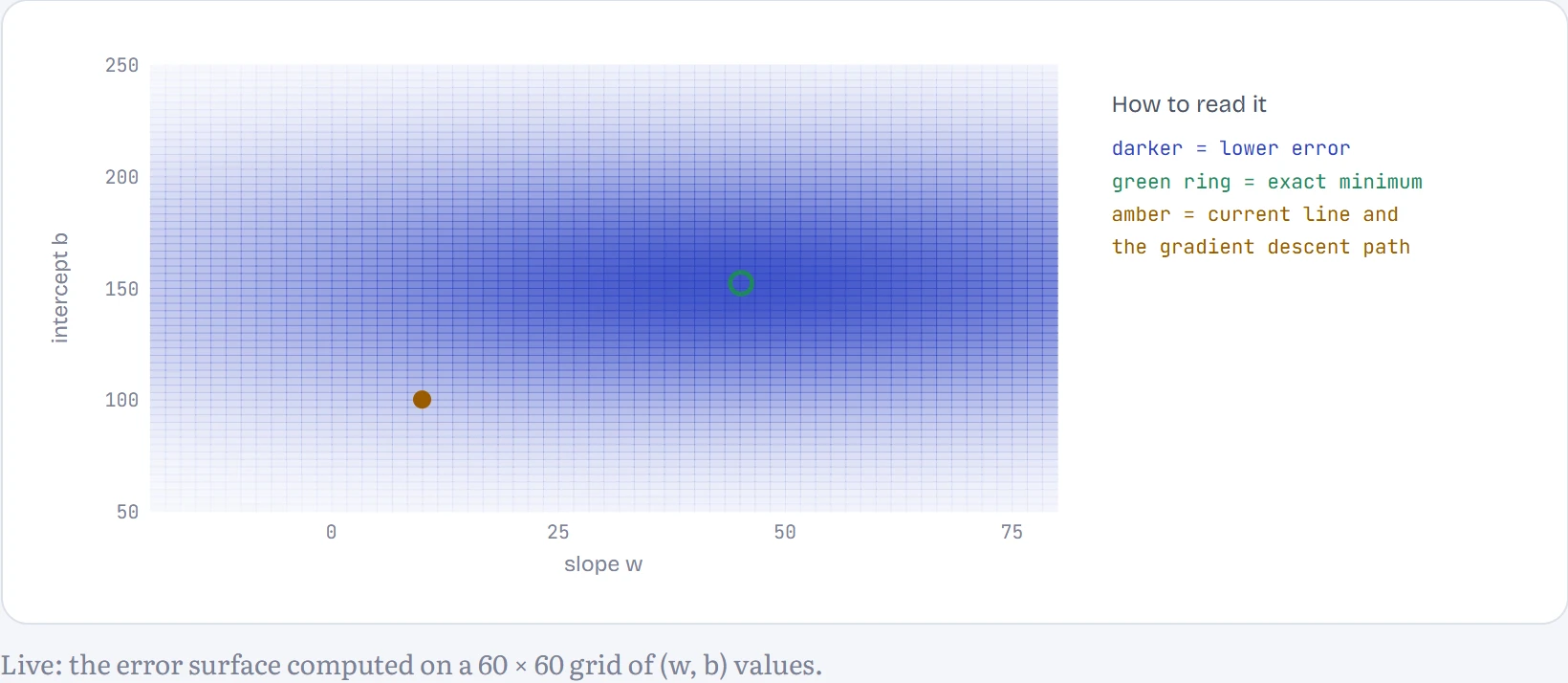
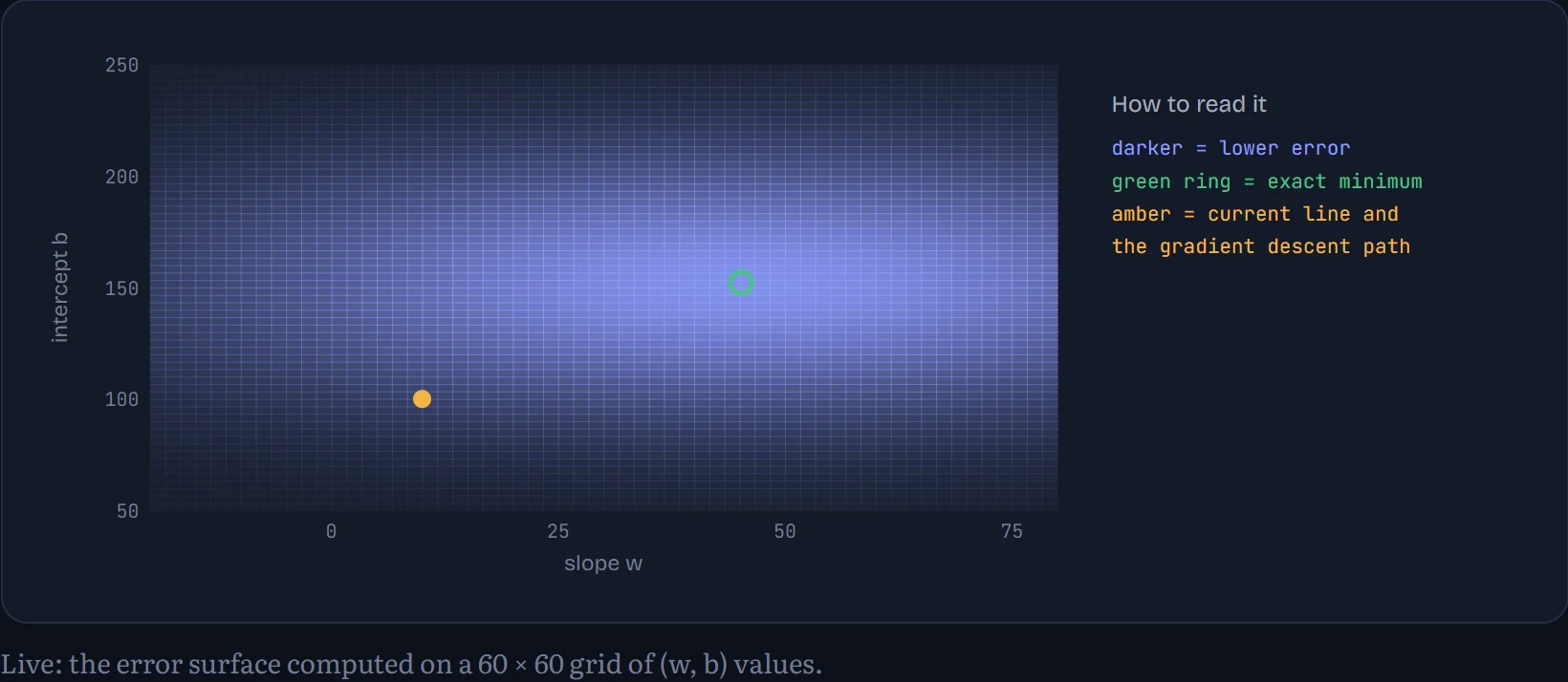
Gradient descent does what Chapter 3 taught: start somewhere, compute which direction is downhill (the gradient, ∂MSE/∂w = (2/n)·Σ(prediction − y)·x and ∂MSE/∂b = (2/n)·Σ(prediction − y)), take a small step that way, repeat. How to read the chart: it's a map of the MSE for every combination of w (across) and b (up), darker where the error is lower, with the path gradient descent took. With a large learning rate it overshoots.
If there's a formula, why bother with gradient descent? Because the formula only exists for a few simple models. The normal equations for a model with n weights need a calculation that grows like n³: fine for 10 weights, hopeless for 10 million. And for anything with a nonlinearity in it, such as every neural network from Chapter 5 on, there's no formula at all. Gradient descent works for any model whose loss you can differentiate, which is why it, and its descendants, train everything from here to the end of the course.
Batches and epochs
Gradient descent as described computes the gradient over every example before taking one step. With 442 patients that's fine; with a billion web pages it means one step per day. The fix is to estimate the gradient from a small random sample, a mini-batch, and step immediately. The estimate is noisy, but it's cheap, and many noisy steps beat a few perfect ones. With a batch of one example it's called stochastic gradient descent (SGD), a name now used loosely for all the mini-batch versions too. One full pass through the dataset is an epoch.
Now the model uses all ten measurements (ten weights plus an intercept). How to read the chart: the loss on all patients against the number of examples looked at, for three batch sizes with the same learning rate.
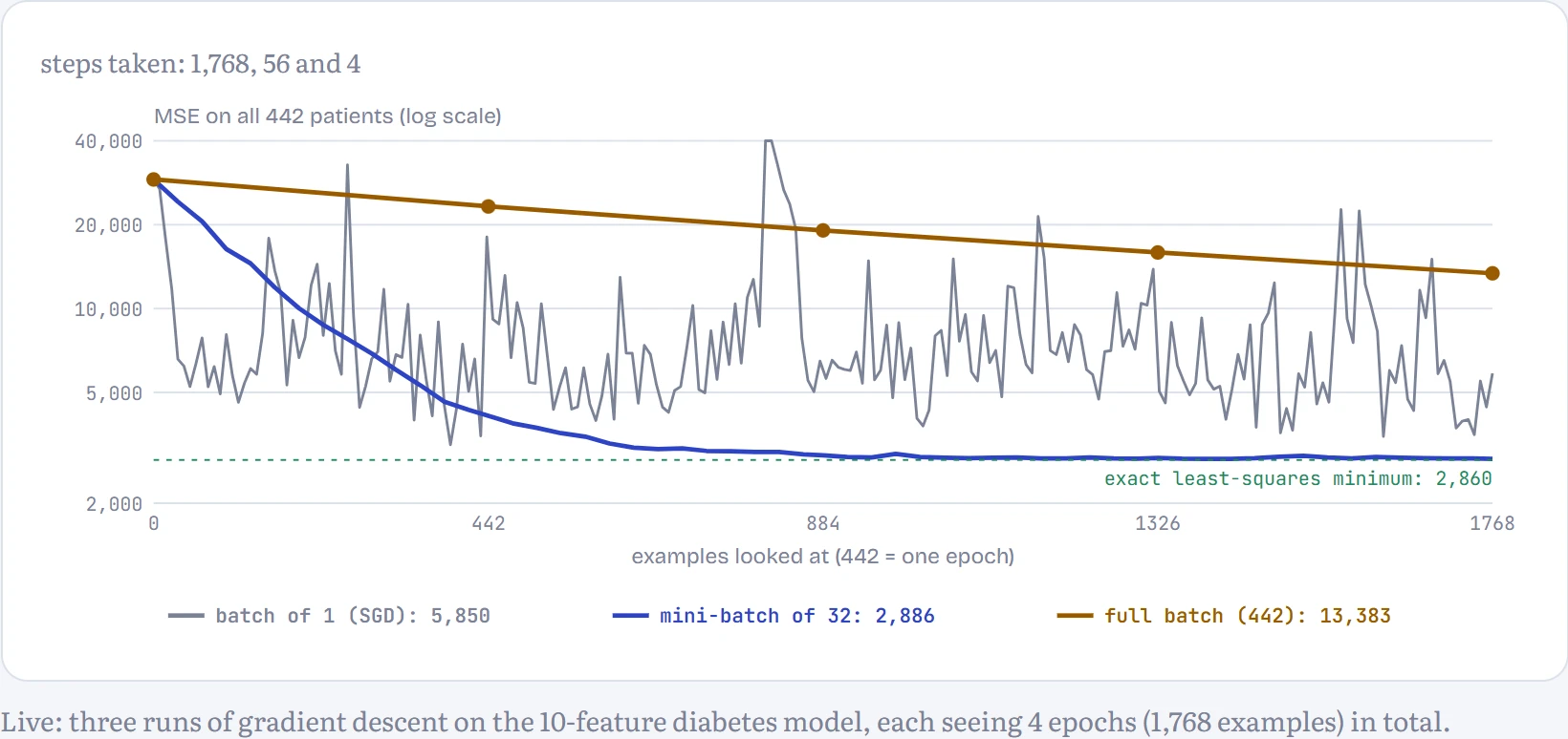
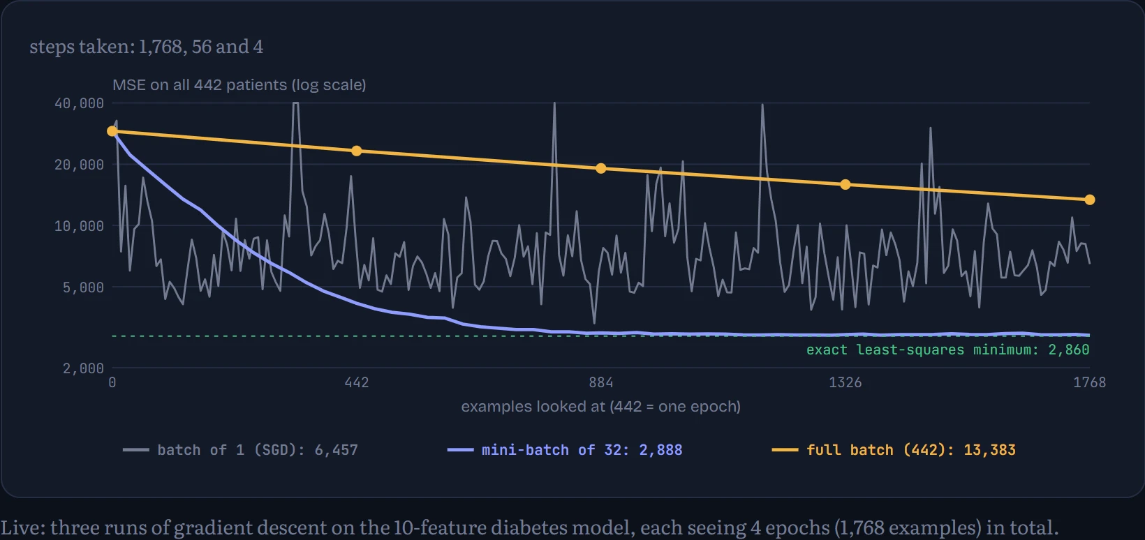
All three runs read exactly the same number of examples. The full-batch run took only 4 steps, each one perfectly aimed, and is still at an error of 13,383, far from the best possible 2,860 (the dotted green line). The mini-batch run took 56 slightly noisy steps and ended at 2,918. Plain SGD took 1,768 very noisy steps: it races down fastest at first, but then can't settle, ending this run at 6,347, because each step chases a single patient, and the learning rate that suits a batch of 32 is too big for steps that noisy. Across reruns: the mini-batch line barely changes, while the SGD line ends somewhere different every time. For the same amount of reading, frequent rough steps beat a few perfect ones, and a modest batch gives most of the speed without the jitter. On a GPU there's a second reason for mini-batches: processing 32 or 1,024 examples at once costs barely more time than processing one, because the hardware works in parallel. Every model from Chapter 5 on trains with mini-batches.
Yes or no: logistic regression
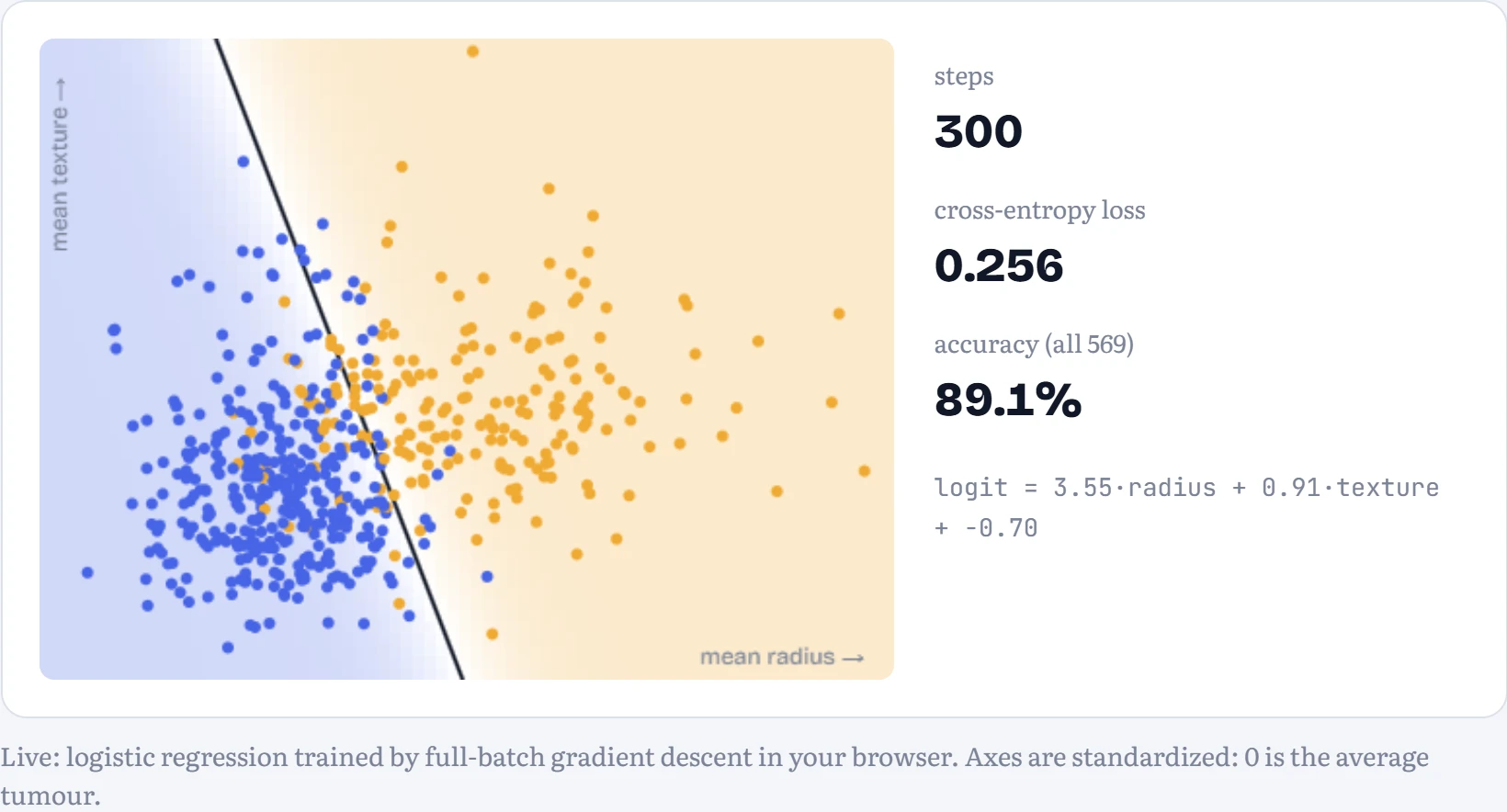
Many questions don't have a number as the answer but a category. Is this tumour malignant? The Wisconsin breast cancer dataset (569 tumours, also bundled with scikit-learn) records 30 measurements of cell nuclei from each biopsy, and whether it turned out malignant. A straight line can't output a probability, because lines run off to infinity. So we keep the linear part and squash it. The linear part, z = w₁x₁ + w₂x₂ + b, is called the logit: any number, positive meaning “probably malignant”. The sigmoid σ(z) = 1 / (1 + e−z) squashes it into a probability between 0 and 1. That's logistic regression, the yes-or-no cousin of the line.
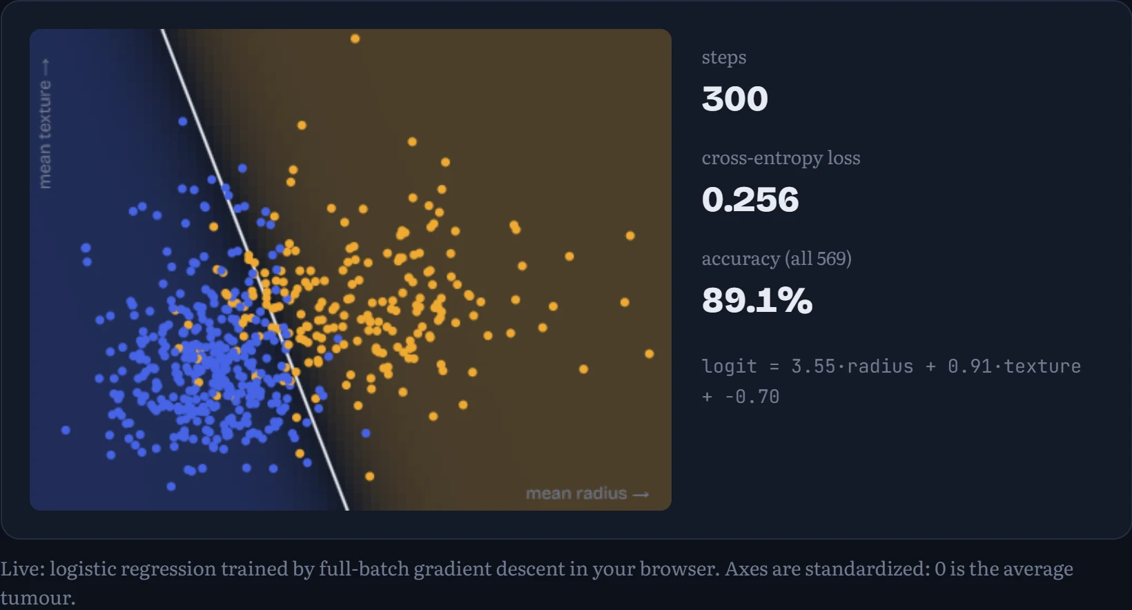
The loss changes too. For each tumour we look at the probability the model gave to what actually happened, and take −log of it: the cross-entropy from Chapter 3. In the figure: the model learning from two of the measurements. Each dot is a tumour (amber = malignant, blue = benign); the background shows the model's probability of malignant, and the line is where it's exactly 50%.
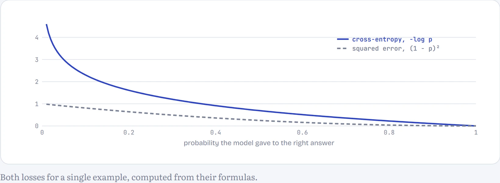
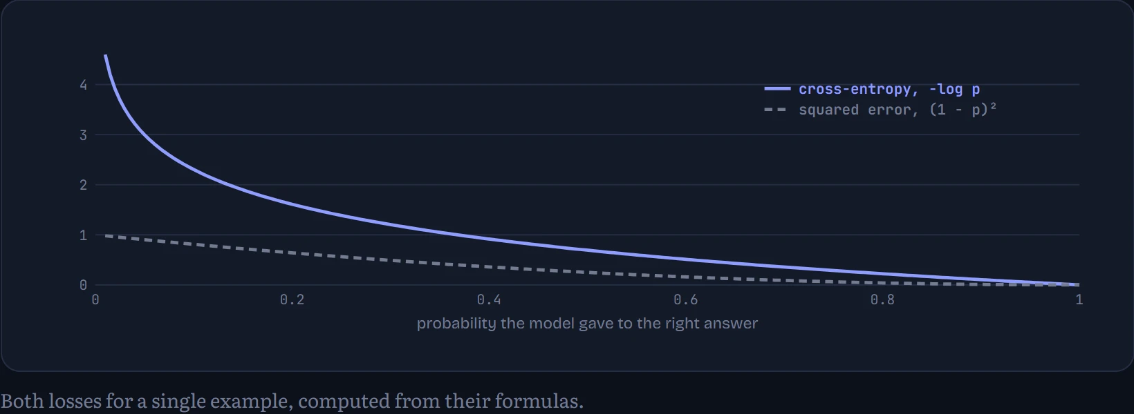
Why −log p instead of squared error? How to read the chart: the loss for one tumour against the probability the model gave to the right answer. When the model is confidently wrong (probability near 0), squared error tops out at 1, a mild scolding; cross-entropy climbs towards infinity. That steep wall is what pushes a classifier to fix its worst mistakes first, and it's also exactly the quantity that maximum likelihood (Chapter 3) tells you to minimize.
Ten digits, one layer: softmax regression
With more than two categories, give each category its own logit and turn the list into probabilities with the softmax: raise e to each logit and divide by the total, so the results are positive and add up to 1. For MNIST's handwritten digits that means 10 logits, each a weighted sum of all 784 pixels plus a bias: 7,850 parameters, no hidden layers. This is softmax regression, and it's exactly the last layer of every classifier and every language model you'll meet, the part that turns scores into a probability for each possible answer.
I trained it on all 60,000 training digits with plain mini-batch gradient descent (3,000 steps of 128 digits, about 6 epochs). It gets 92.2% of the 10,000 test digits right (92.5% on the training digits), with no hidden layer at all. Because it's so simple, you can look straight at what it learned: each digit's 784 weights can be laid out as a 28 × 28 picture.
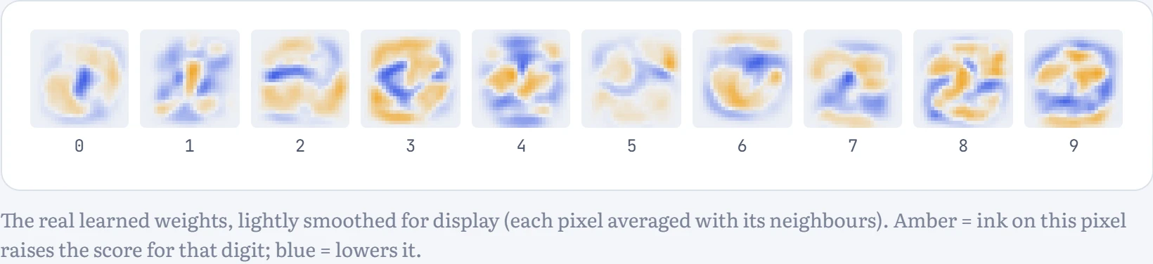
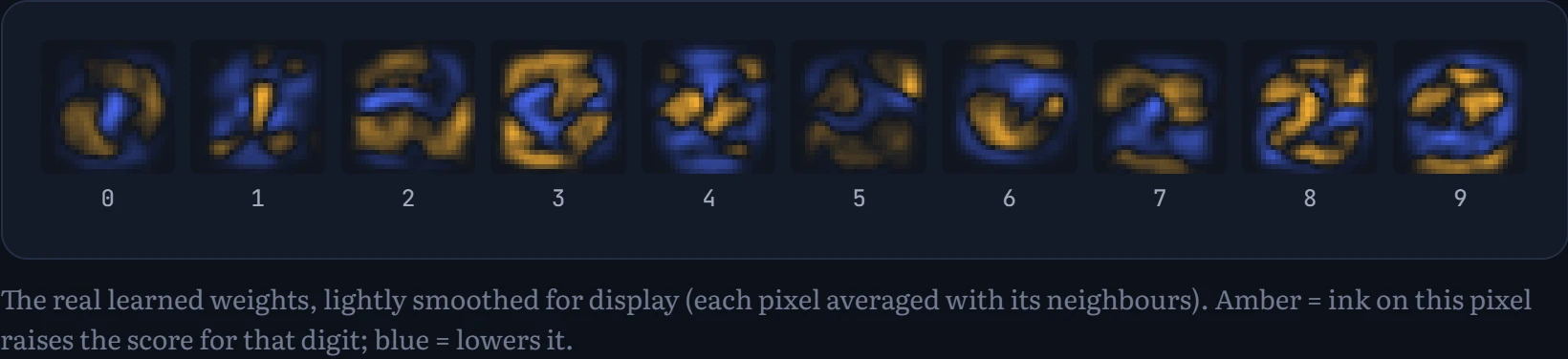
How to read the templates: each image is one digit's 784 weights laid out as a picture. The model has learned a rough stencil for each digit: amber where that digit's strokes usually are, blue where ink argues against it (look at the blue hole in the middle of the 0, where a 0 has no ink). Classification is just asking which stencil your drawing overlaps best.
How much data does it need? How to read the chart: I trained the same model on random subsets of the training set, from 100 digits to all 60,000, and measured accuracy on the training digits and on the 10,000 test digits it never saw.
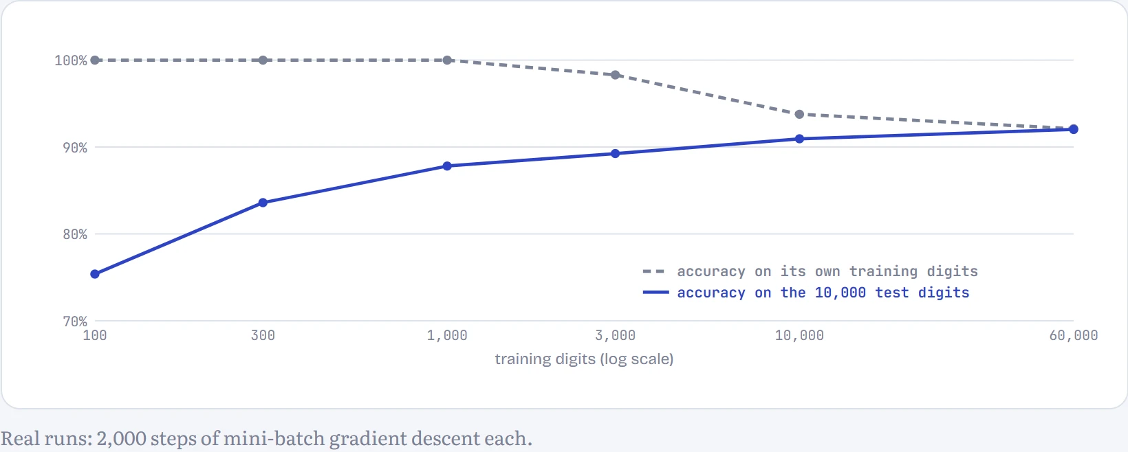
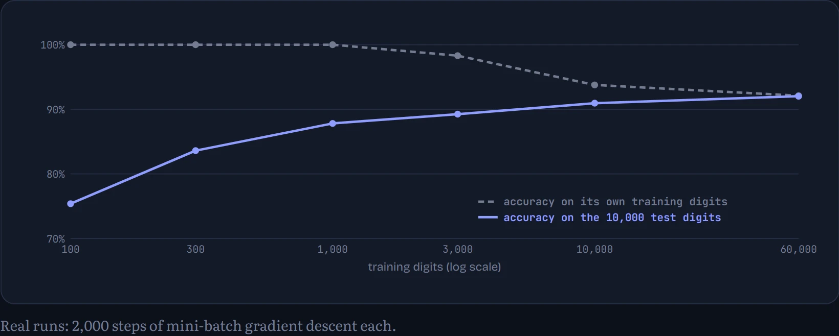
With 100 training digits the model gets every one of them right (100%) and only 75% of the test digits: it has 7,850 adjustable numbers and only 100 examples, so it can fit them perfectly, including their quirks. As the training set grows the two lines converge. With all 60,000, training accuracy (92.1%) and test accuracy (92.0%) are almost the same: the model can no longer memorize, and it's now limited by how simple it is, not by data. The gap between the lines is the signature of overfitting, and closing it is the next section's subject.
Overfitting: learning versus memorizing
A model's real job is to do well on data it hasn't seen. Score on training data alone and you'll reward memorization. So before training, split the data three ways: a training set to fit the parameters, a validation set to choose hyperparameters and decide when to stop, and a test set locked away until the very end, used once, for the number you report. Every time you look at the test set and change something, it leaks a little information into your choices and stops being an honest estimate.
Here's the classic picture. Twelve points from a smooth curve plus noise, fitted by polynomials of increasing degree (degree 1 is a line, degree 2 a parabola, and so on). In the figure: the fit (left) and the errors (right) for a polynomial of a chosen degree: training error on the 12 points, and test error on 200 fresh points from the same curve. Weight decay , a penalty on large weights, can be added too; we'll come back to it.
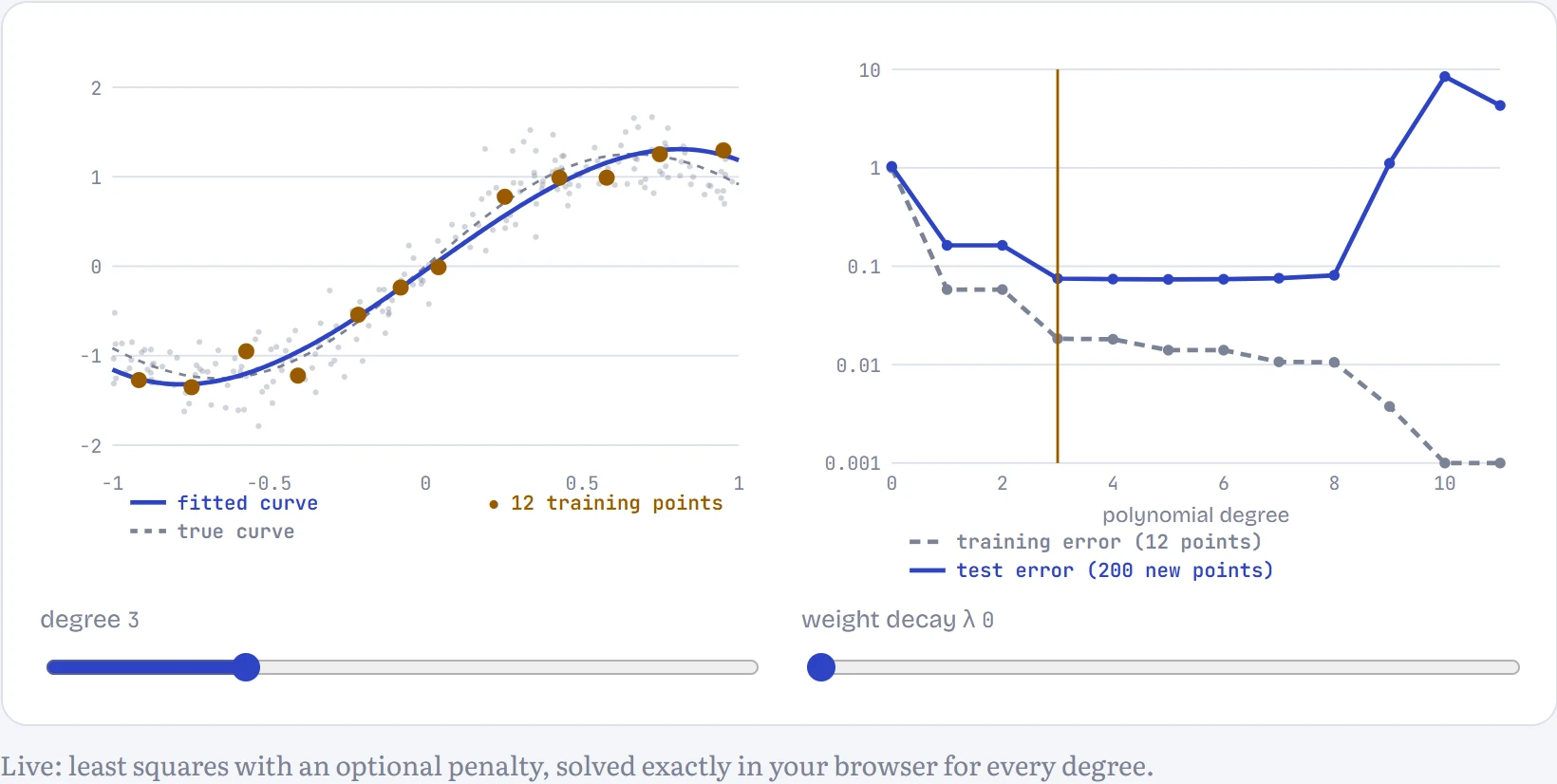
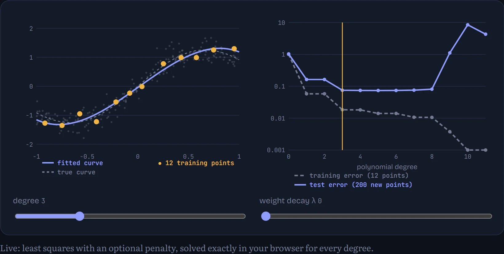
Right now: degree 3: training error 0.018, test error 0.075. This is near the sweet spot. At this λ the lowest test error is at degree 5 (0.074). Raise weight decay at a high degree: the penalty tames the swings without removing the flexibility, and test error comes back down.
This trade-off has a name: bias versus variance. A model that's too simple is wrong in a consistent way whatever data you give it (high bias: the line can't bend). A model that's too flexible fits whatever noise happens to be in its particular sample, and would fit a different sample completely differently (high variance). The best model sits between. Two standard tools push a flexible model back towards the middle: weight decay adds λ × (sum of squared weights) to the loss, so wild curves with huge coefficients cost extra (it's the prior from Chapter 3's MAP estimate in disguise), and early stopping simply stops training when the validation loss stops improving.
Both show up in a real network. I trained a neural network (two hidden layers of 256 units, about 270,000 parameters, the kind you'll build in Chapter 5) on just 1,000 handwritten digits, for 150 passes through them, with three strengths of weight decay. How to read the chart: loss on the 1,000 training digits (dashed) and on 5,000 validation digits (solid), per epoch; the dot marks the epoch with the lowest validation loss, where early stopping would have stopped.
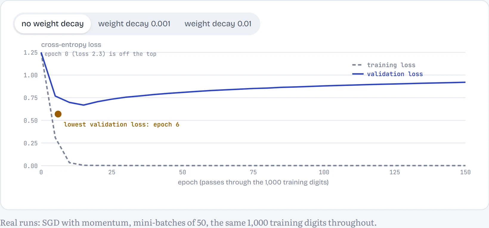
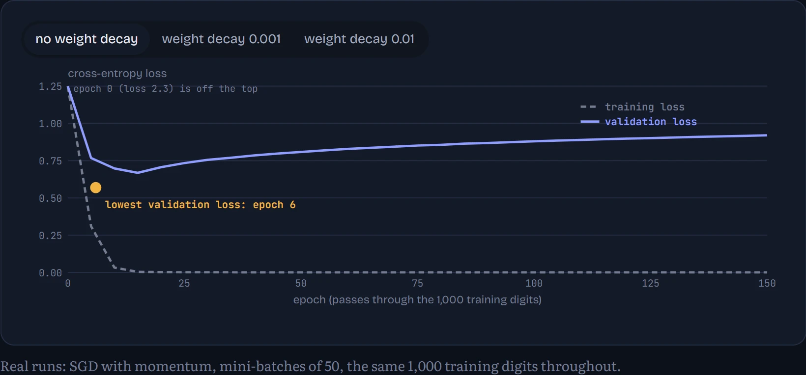
Without weight decay, training loss drops to almost zero: the network memorizes all 1,000 digits. Validation loss bottoms out at epoch 6 and then climbs for the rest of the run. Here's the twist that real training throws at you: validation accuracy didn't follow. It was 84.3% at epoch 6 and 86.3% at the end. The network kept getting slightly better at picking the right digit while becoming wildly overconfident when wrong, and cross-entropy punishes confident mistakes hard. So “when to stop” depends on what you care about: stopping at the lowest validation loss gives better-calibrated probabilities; stopping at the best validation accuracy gives more right answers. The measuring section shows how overconfident the unregularized network got.
With weight decay 0.01, the picture changes: validation loss keeps improving almost to the end (lowest at epoch 146) and finishes at 86.1% accuracy. The penalty stops the weights growing large enough to memorize with total confidence. Neither run can beat the basic problem, though: 1,000 examples is not much, and the softmax regression trained on all 60,000 digits (92.2%) beats this far bigger network trained on 1,000. More data is the most reliable fix for overfitting there is.
The sneakiest failure isn't overfitting, it's leakage: information from the test set getting into training, so the score looks better than the model is. It happens more easily than you'd think. Normalizing features using statistics computed on all the data, before splitting. Duplicates or near-duplicates that land on both sides of the split. Splitting a patient's scans randomly, so the same patient appears in training and test. Predicting next month's sales with a feature that was only recorded after the sale. For language models it's called contamination: benchmark questions that appeared in the training text. Chapter 15 measures it, and finds that a model which saw the test questions can look dramatically better than it is.
Continue the lesson
The whole lesson, with its drawings and its questions. 5 more sections after the ones above.