
Subword tokenization and embeddings: BPE, WordPiece and word2vec skip-gram
Text is already numbers, as Unicode code points stored in UTF-8 bytes, just not useful ones. Byte-pair encoding builds a vocabulary by repeatedly merging the most frequent pair of symbols, and an embedding table turns each token into a learned vector. word2vec learns those vectors by predicting a word's neighbours.
What this page answers
How does byte-pair encoding work?
It starts from single characters or bytes and repeatedly merges the most frequent neighbouring pair into a new token, one merge at a time, until the vocabulary is the size you want. Read it in “Byte-pair encoding, one merge at a time”
Why must text be Unicode-normalized before tokenizing?
Because the same visible character can be stored two ways, such as one code point for é or an e followed by a combining accent. Without normalizing, the same word gets split differently depending on how it was typed. Read it in “Text is already numbers (just not useful ones)”
Text is already numbers (just not useful ones)
Your computer stores every character as a number. Unicode gives each character a code point (“A” is 65, “é” is 233, “東” is 26,481), and UTF-8 stores each code point as one to four bytes. English letters fit in one byte. Accented letters take two, most Asian scripts three, emoji four.
Look at what's really underneath your text:
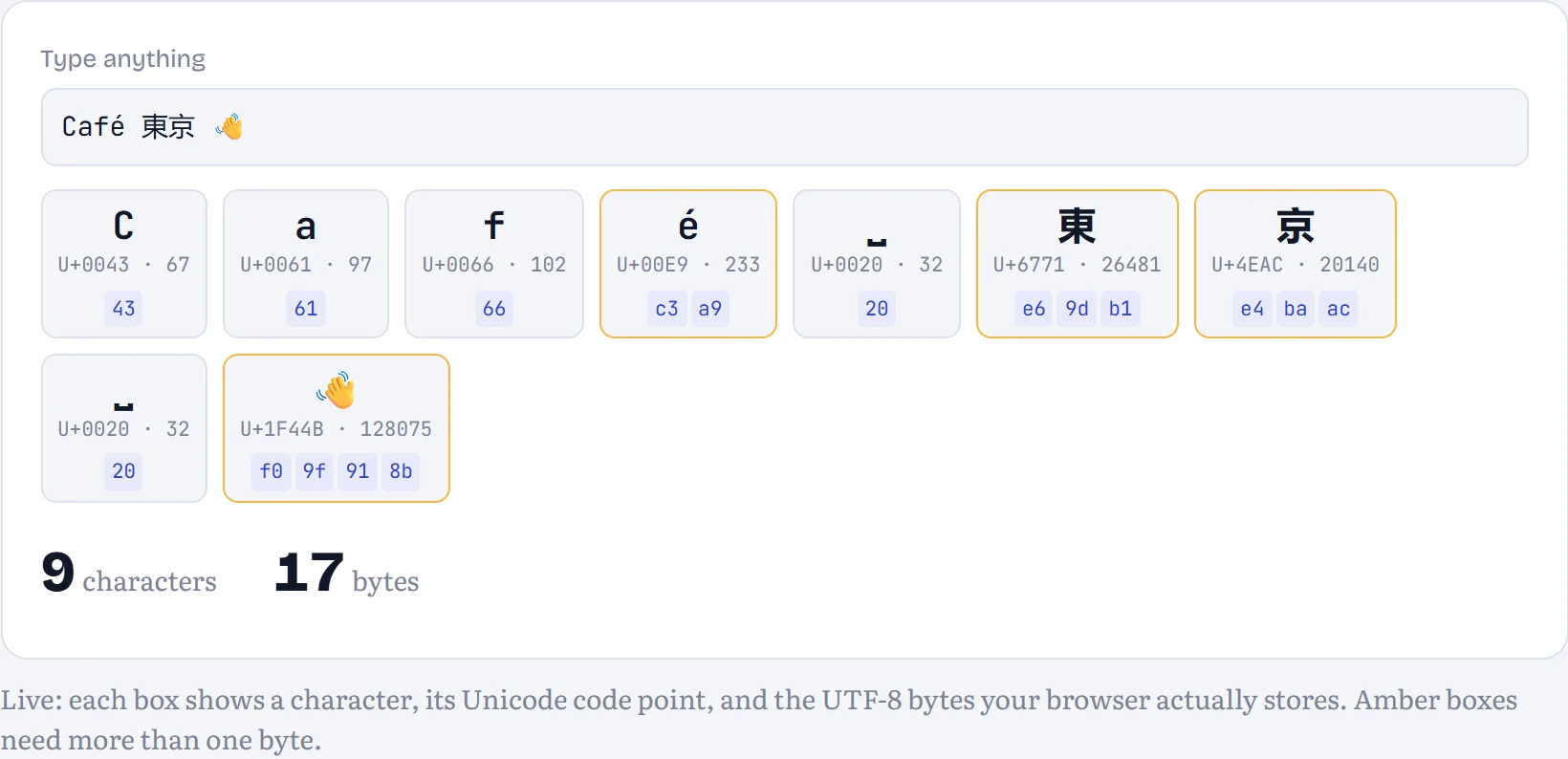
Predict first. Here are two strings: café and café. They look identical. Are they the same sequence of bytes?
- Yes, obviously
- Not necessarily
Answer. Not necessarily, and these two aren't. Measured right now in your browser: the first is 5 bytes, the second 6; our tokenizer turns them into 5 and 5 tokens; after NFC normalization they're identical: true. Unicode lets “é” be stored as one code point, or as “e” followed by a combining accent. To a model, those are different inputs. That's why text pipelines normalize first (usually to the composed form, NFC). Skip it, and the same word gets split differently depending on which keyboard typed it.
From raw files to a training corpus
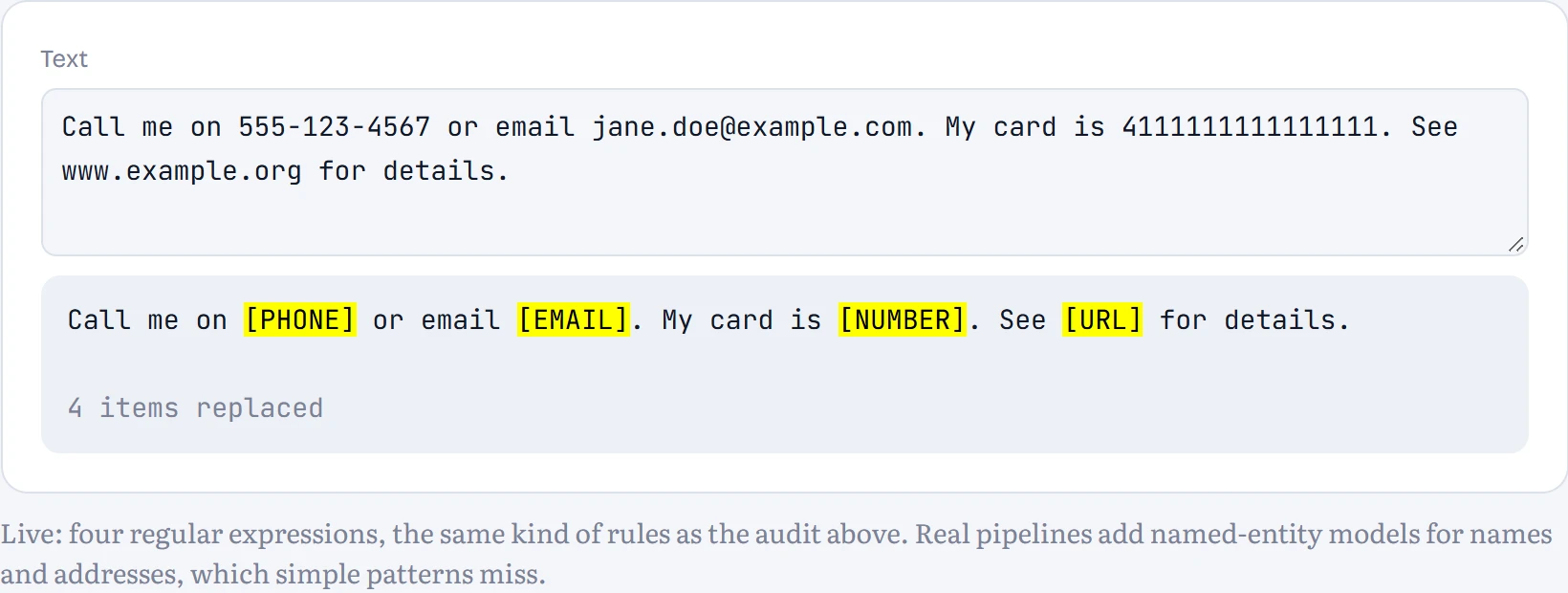
Before any tokenizer sees it, raw text goes through a pipeline: decode the bytes, normalize Unicode, drop junk, remove duplicates, scrub personal data, and split into training and test sets. What each step finds depends entirely on the source. I ran a simple audit over the raw TinyStories validation file used throughout this course. How to read the table: what each check found.
| Check | Found |
|---|---|
| Stories in the file | 27,630 (22.5 million characters, median 719 per story) |
| Characters outside plain ASCII | 4,613, in 726 stories. Most common: right double quotation mark (1642), left double quotation mark (1630), right single quotation mark (1183), en dash (69), left single quotation mark (38) |
| Stories changed by Unicode normalization | NFC: 0 · NFKC (also folds look-alike characters): 7 |
| Exact duplicate stories | 0 |
| Very short stories (under 200 characters) | 0 |
| Possible personal data | email address: 0 · phone number: 0 · web address: 0 · long number (ID, card): 0 |
This file is unusually clean, and that's the first lesson: TinyStories was written by a language model on purpose, so it has no duplicates, no very short fragments and nothing resembling personal data, and only 2.6% of stories contain anything beyond plain ASCII, mostly typographic quotes and dashes. Run the same checks on scraped web text and every row lights up: Chapter 10 shows the quality filters and near-duplicate detection that web corpora need. The audit also caught one subtle splitting question. If you split the corpus into training and test sets line by line, instead of story by story, then 0.4% of test lines appear word for word in training, against 0.3% when whole stories go to one side. The difference is small here only because lines like “The end.” (235 times) are the main repeats. For data with many repeated lines, such as code, chat logs or forum threads, splitting by document, user or date is what keeps a test set honest.
In the figure: The scrubber runs the same kind of rules a pipeline uses to find personal data and replace it with placeholders before training.
Licensing and ethics come before any of this. Every text has an owner and terms. Public-domain works (Shakespeare, most books published before about a century ago) can be used freely. Openly licensed text (Wikipedia, many code repositories) comes with conditions such as attribution or sharing derivatives under the same terms. Much of the web is simply copyrighted, and whether training on it is allowed is being argued in courts around the world right now. Datasets like TinyStories publish their own license on their dataset card; read it before you build a product on it. Beyond the law: text can contain personal information people never agreed to share, and a model trained on it can reproduce it (Chapter 10 measures how repetition causes memorization). It also absorbs the biases of whoever wrote the text. A responsible pipeline records where every source came from, honours opt-outs, scrubs personal data, and documents what's in the mix.
Choosing the unit: a three-way tug of war
So which numbers should a model see? You could feed it raw bytes, or characters, or whole words. Each choice pulls on three things at once: how big the vocabulary is, how long the sequences get, and what happens to text the model has never seen. Here are the real numbers on our Shakespeare corpus:
| Unit | Vocabulary size | Tokens per character | Characters per token | Held-out tokens never seen in training |
|---|---|---|---|---|
| Bytes | 256 | 1.00 | 1.00 | 0% |
| Characters | 65 | 1.00 | 1.00 | 0% |
| Subwords (BPE, 2,256) | 2,256 | 0.38 | 2.61 | 0% |
| Words (every training word) | 13,461 | 0.18 | 5.50 | 6.5% |
| Words (top 3,000 only) | 3,000 | 0.18 | 5.50 | 15.1% |
Reading the table: “tokens per character” is how long sequences get (lower means shorter, which is cheaper for the model). “Held-out tokens never seen in training” is the share of tokens in new text that the vocabulary simply doesn't contain, so the model can't handle them at all (lower is better, and zero is the goal).
Words look great until you check the right-hand column: validation text is full of words the training text never contained, and a word-level model is simply stuck on them. Characters never get stuck, but every sentence becomes a long string of tiny steps, and attention's cost grows with the square of the length (lesson 8.4). Subword tokenization splits the difference: common words become a single token, rare words fall apart into familiar pieces, and nothing is ever unknown because, worst case, it falls all the way back to bytes.
The standard way to build that subword vocabulary is a beautifully dumb algorithm from data compression.
Byte-pair encoding, one merge at a time
Start with every word split into single symbols. Count every pair of neighbouring symbols across the whole text. Glue the most frequent pair into a new symbol. Repeat. That's the entire training algorithm. The list of merges, in order, is the tokenizer.
It's like a person inventing shorthand while copying out a long text. You notice you keep writing “t” then “h”, so you invent a single squiggle for “th”. Then you notice “th” followed by “e” is everywhere, so “the” gets its own squiggle. Each new squiggle is chosen because it saves the most writing right now. After a few thousand of them, common words are one squiggle each, and rare words are spelled out from smaller squiggles.
How to read it: the left side shows how the training text is currently split, one chip per symbol, and the vocabulary learned so far (the newest symbol highlighted). The right side counts every pair of neighbouring symbols; the highlighted top row is the pair the next Merge will glue together. Merge by merge, it discovers structure nobody told it about.
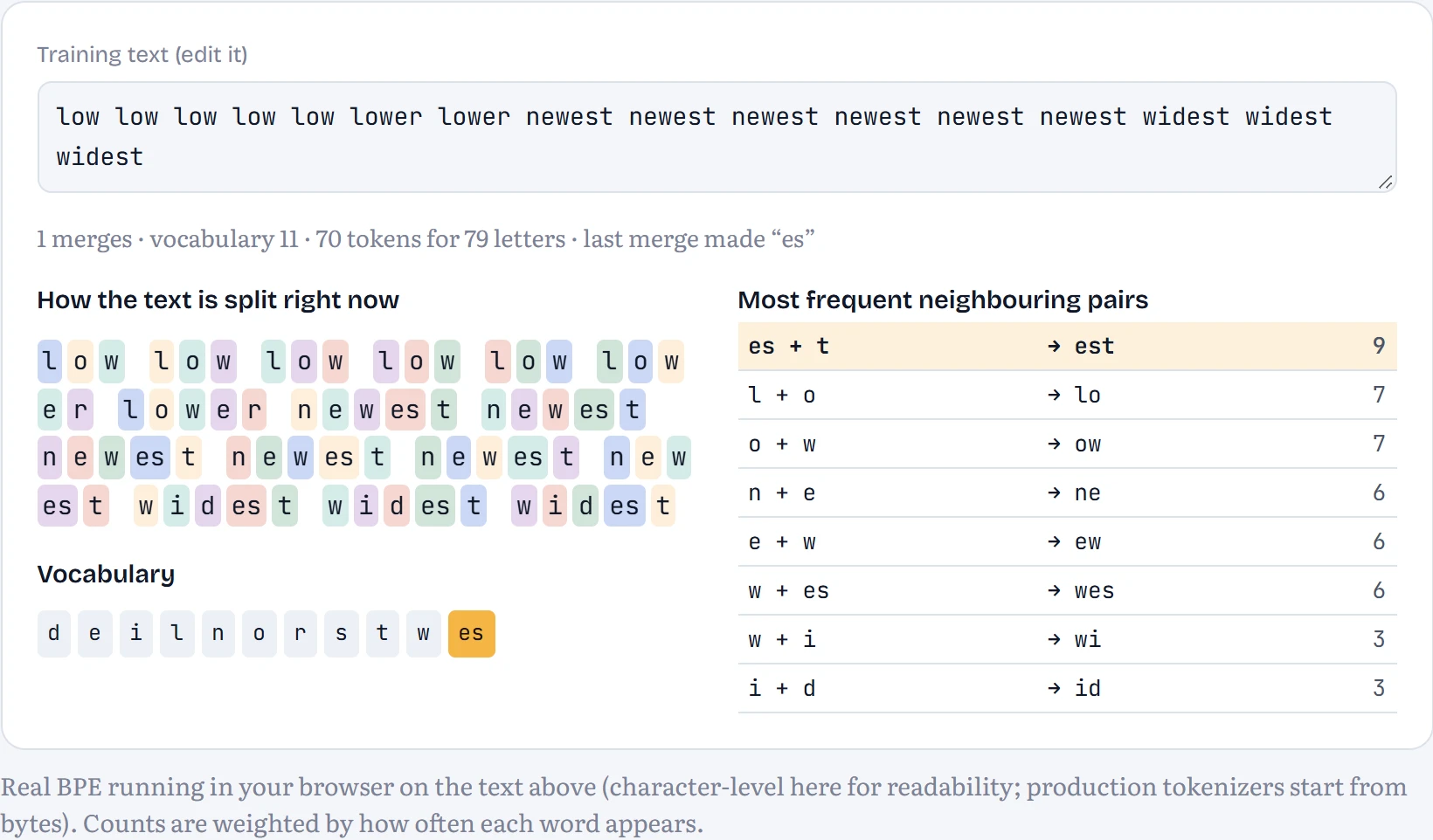
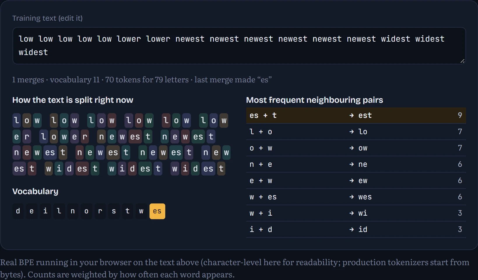
On the default text it first finds “es”, then “est”, so the suffix of newest and widest becomes one reusable piece. Then “lo” and “low”. Nobody told it about morphology; frequency alone found it. Encoding new text later replays the merges in the order they were learned, so a word the tokenizer never saw, like “lowest”, comes out as familiar pieces: “low” + “est”.
The real thing: 2,000 merges on all of Shakespeare
The tokenizer at the top of the page was trained exactly this way, starting from the 256 possible byte values, on the 1,003,854-character training split. Here are the first 30 merges it chose, in order (a dot · marks a space):
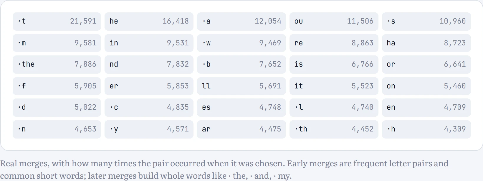
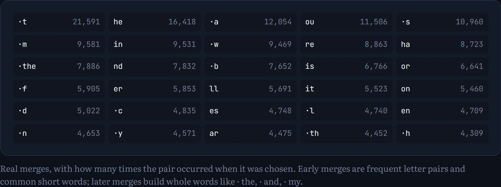
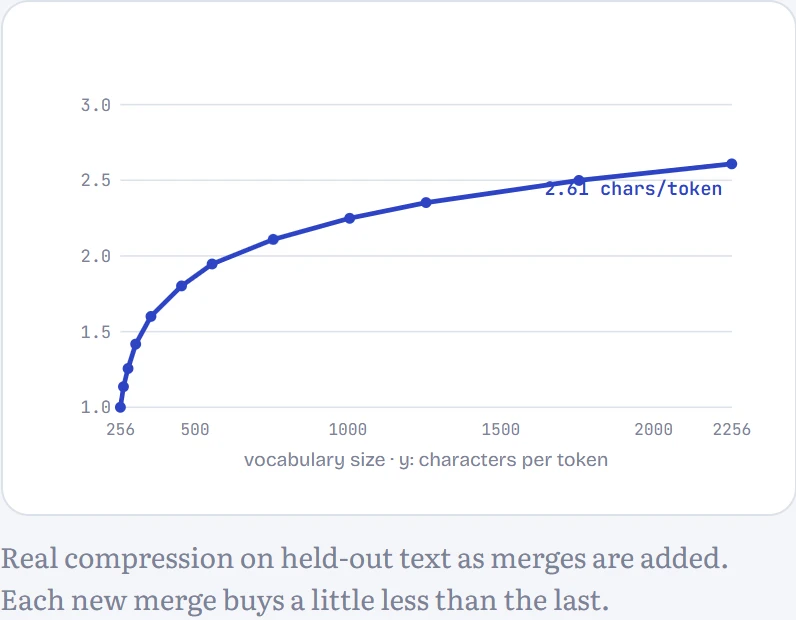
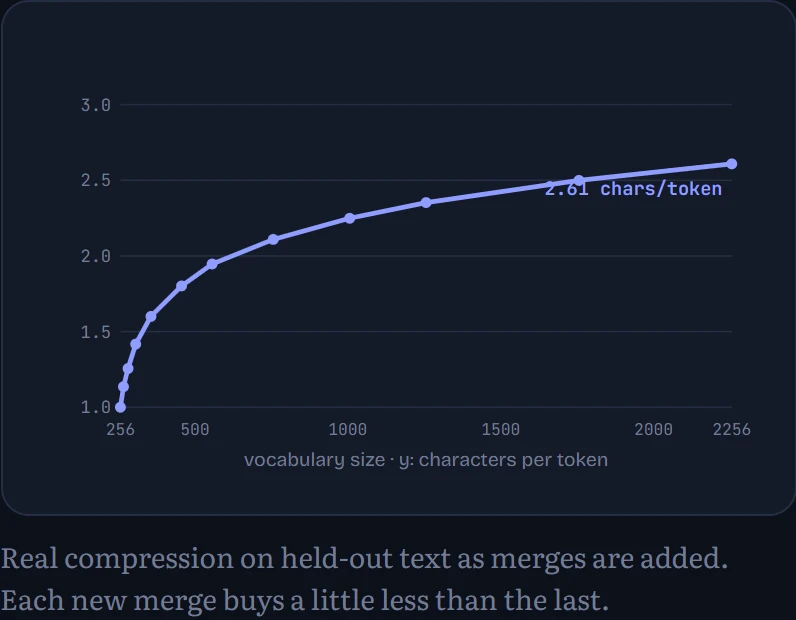
How much does all this merging actually buy? The chart below measures it on text the tokenizer never trained on. How to read it: at the far left, with just the 256 byte values, each token covers about one character. Every merge lets a token cover a little more, so the line climbs, but it flattens out: the first merges glue together extremely common pairs and save a lot, while later ones target rarer patterns and save less. Next to it is a well-known puzzle that tokenization explains.
Predict first. Ask a chatbot “how many r's are in strawberry?” and models have famously answered wrong. Look at how our tokenizer splits it, then guess why.
Answer. The model never sees letters. It sees token IDs, and the ID for a piece like ber or ry doesn't spell itself out. Counting letters means the model has to have memorized the spelling of every token, which it only partly does. Numbers have a related problem. Our Shakespeare tokenizer saw so few digits that 1234567 stays as seven single digits; tokenizers trained on code and maths merge digits into chunks, often up to three at a time, and those chunks don't line up with place value the way column arithmetic needs.
WordPiece: the same idea, a different rule for choosing merges
BPE isn't the only subword method. WordPiece, used by BERT and many models derived from it, also starts from characters and merges pairs, but it chooses differently. BPE merges the most frequent pair. WordPiece merges the pair whose merge most increases the likelihood of the training text, which works out to count(ab) ÷ (count(a) × count(b)): it prefers pairs that occur together far more often than their parts occur separately. It also marks pieces that continue a word with ##, so “playing” might become play ##ing. To compare them fairly, I trained both on the same words from the Shakespeare training split, to the same vocabulary size, and measured them on held-out text. How to read the table: how each splits a few words, and the average number of tokens per held-out word (fewer means each token carries more).
| Word | BPE | WordPiece |
|---|---|---|
| the | the | th · ##e |
| thee | thee | th · ##e · ##e |
| king | king | king |
| kingdom | king · dom | king · ##d · ##o · ##m |
| unkindness | un · kind · ness | un · ##k · ##i · ##n · ##d · ##n · ##e · ##s · ##s |
| wherefore | where · fore | wh · ##e · ##r · ##e · ##f · ##o · ##r · ##e |
| strawberry | stra · w · ber · ry | s · ##t · ##r · ##a · ##w · ##b · ##e · ##r · ##r · ##y |
| tokenization | to · ken · i · z · ation | to · ##k · ##e · ##n · ##iz · ##a · ##t · ##i · ##o · ##n |
| Romeo | Romeo | Rom · ##e · ##o |
| antidisestablishmentarianism | an · ti · dis · est · a · bl · ish · ment · ar · i · an · is · m | a · ##n · ##t · ##i · ##d · ##i · ##s · ##e · ##s · ##t · ##a · ##b · ##l · ##ishm · ##e · ##n · ##t · ##a · ##r · ##i · ##a · ##n · ##i · ##s · ##m |
| Tokens per held-out word | 1.55 | 3.30 |
The two rules learn very different vocabularies. BPE's first merges were the most common letter pairs (th, ou, er, in, an, the). WordPiece's were ##DW, EDW, ##MP, ##XF, OXF, OF: pieces of rare, all-capital speaker names like EDWARD, because letters that almost never appear apart score highest under its rule. With a small vocabulary of 500 tokens, that cost WordPiece dearly on ordinary words: 4.09 tokens per word against BPE's 2.00. At 2000 tokens the gap remains: 3.30 against 1.55. Real WordPiece vocabularies are much larger (BERT's has 30,000 entries) and are trained on lower-cased text when the model is “uncased”, which removes exactly the capital-letter names that dominated here. Neither method is wrong; they optimize different things, and the choice changes what the model sees. A third method, the unigram language model used by SentencePiece, works the other way round: it starts from a huge vocabulary and prunes the pieces that matter least.
Every language pays a different price
Our tokenizer learned only English Shakespeare. Anything else falls back toward raw bytes. Here's the same greeting in several languages, tokenized live:
| Language | Text | Characters | Tokens | Tokens vs English |
|---|---|---|---|---|
| English | Good morning, my friend. How are you today? | 43 | 13 | 1.0× |
| French | Bonjour, mon ami. Comment vas-tu aujourd'hui ? | 46 | 28 | 2.2× |
| German | Guten Morgen, mein Freund. Wie geht es dir heute? | 49 | 27 | 2.1× |
| Hindi | सुप्रभात, मेरे दोस्त। आज आप कैसे हैं? | 37 | 95 | 7.3× |
| Japanese | おはよう、友よ。今日の調子はどう? | 17 | 51 | 3.9× |
| Arabic | صباح الخير يا صديقي. كيف حالك اليوم؟ | 36 | 65 | 5.0× |
OPEN RESEARCH. Production tokenizers are trained on multilingual data, which narrows these gaps but doesn't close them: the same sentence can still cost several times more tokens in some languages than in English. More tokens means higher API cost, less text fitting in the context window, and potentially worse model quality for those languages. How to make tokenization fairer, or skip it entirely with byte-level models, is an active research question.
Embeddings: a learned lookup table
A token ID is just a name tag. ID 1047 isn't “bigger” than ID 12, and you can't do arithmetic on names. So the first thing every language model does is look each ID up in a table: row 1047 of a big matrix, a vector of a few hundred numbers. You met this in Chapter 2: picking row i is the same as multiplying a one-hot vector by the matrix, minus all the wasted multiplications by zero.
The table starts random. Training adjusts its rows like any other weights, and since words used in similar ways get similar gradients, their rows drift together. The cleanest place to watch that happen is word2vec.
Imagine placing everyone at a big party on a map, with no information except who they keep chatting with. People who hang around the same groups end up close together, even if you never learn their names or jobs. Embeddings do this for words: a word's position (its vector) is learned purely from which other words it keeps appearing next to. Words that turn up in the same company, like king and duke, end up near each other.
word2vec: predict the neighbours
The skip-gram trick is to invent a fake task whose only purpose is to shape the table. For each word in the text, try to predict the words within a few positions of it. A full softmax over thousands of words for every pair would be slow, so negative sampling turns it into yes/no questions instead: “Is crown really near king?” should score high; “Is pudding near king?”, with pudding picked at random, should score low.
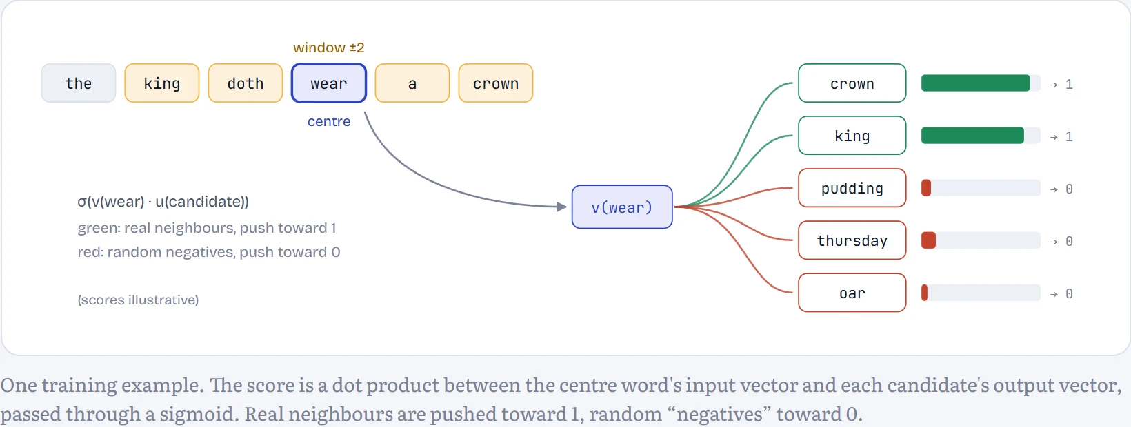
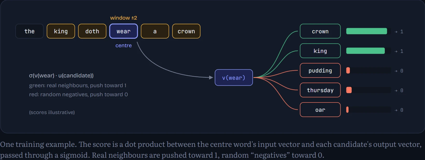
Repeat that a few million times and words that keep turning up in the same company end up with vectors pointing the same way. Nothing in the objective says “meaning”. It falls out of where words appear, which is the distributional hypothesis from Chapter 2.2, now learned instead of counted.
Continue the lesson
The whole lesson, with its drawings and its questions. 6 more sections after the ones above.