
Probability, entropy and cross-entropy, and gradient descent on computational graphs
A language model is a table of conditional probabilities, learned by estimation. Cross-entropy measures how surprised the model is by the real next token, and that number is the loss. Derivatives say which way is downhill, gradients flow back through a computational graph, and gradient descent follows them to a lower loss.
What this page answers
What is the difference between joint, marginal and conditional probability?
Joint P(a, b) is the share of all pairs that are exactly a then b. Marginal P(a) ignores the partner. Conditional P(b | a) asks, of the pairs that start with a, what share continue with b. A language model needs the conditional. Read it in “Probability, from counting”
What is cross-entropy loss?
The average surprise of the model at what really came next. It is the loss a language model is trained to minimise. Read it in “Surprise, entropy and cross-entropy”
Probability, from counting
A probability is a number between 0 and 1 saying how much of the time something happens. The most honest way to get one is to count. I took 2,000 stories from TinyStories (a dataset of simple children's stories written to train small language models) and counted every pair of neighbouring characters. That table of counts is your Chapter 1 bigram model, and it holds three different kinds of probability, which people mix up all the time.
The joint probability P(a, b) is the share of all pairs that are exactly “a then b”. The marginal probability P(a) ignores the partner: add up a whole row. The conditional probability P(b | a), read “b given a”, is what a language model needs: of the pairs that start with a, what share continue with b? It's one cell divided by its row's total. In the figure: each cell of the grid is a joint probability (darker = more common), for the letters and the space.
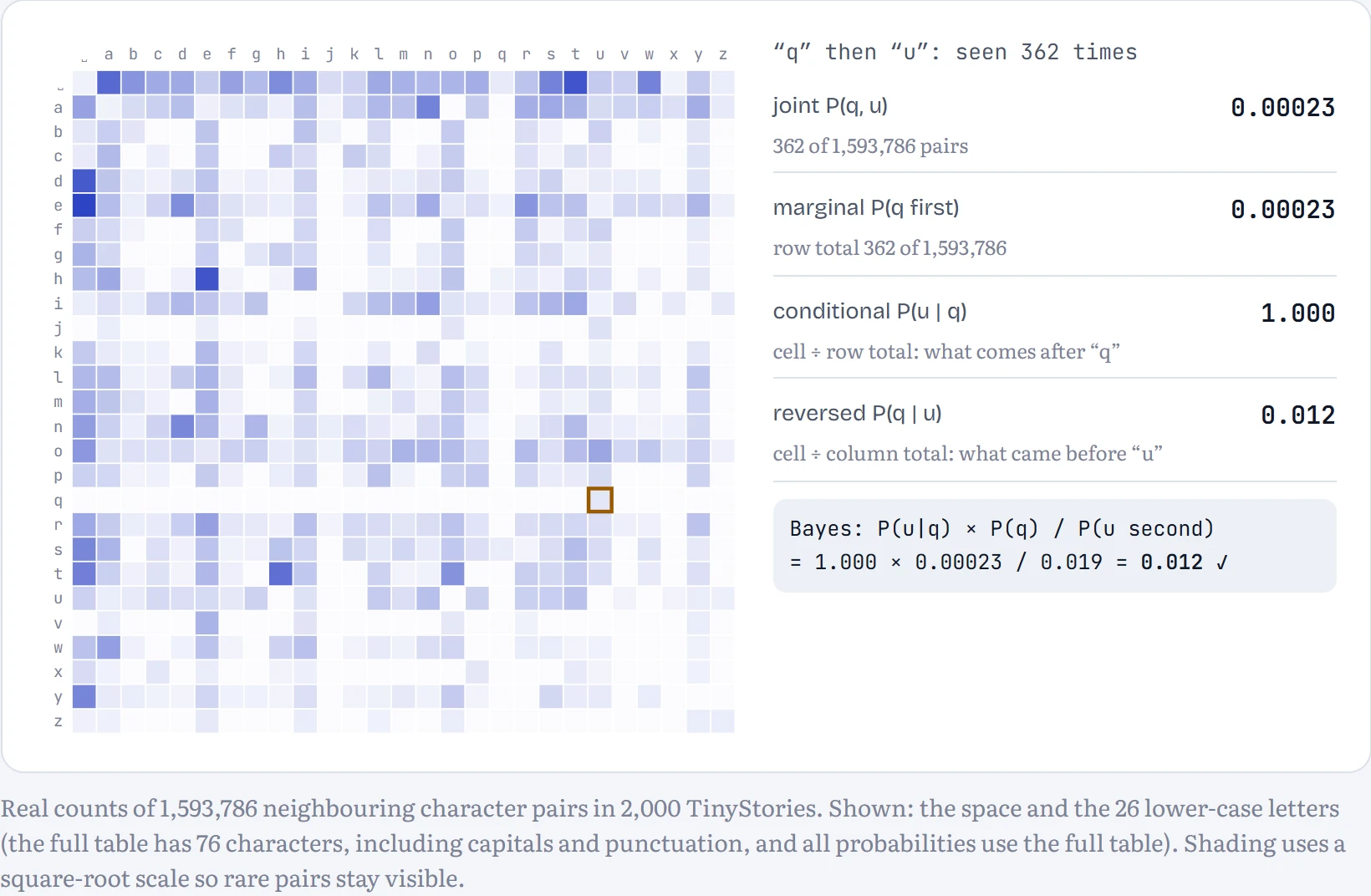
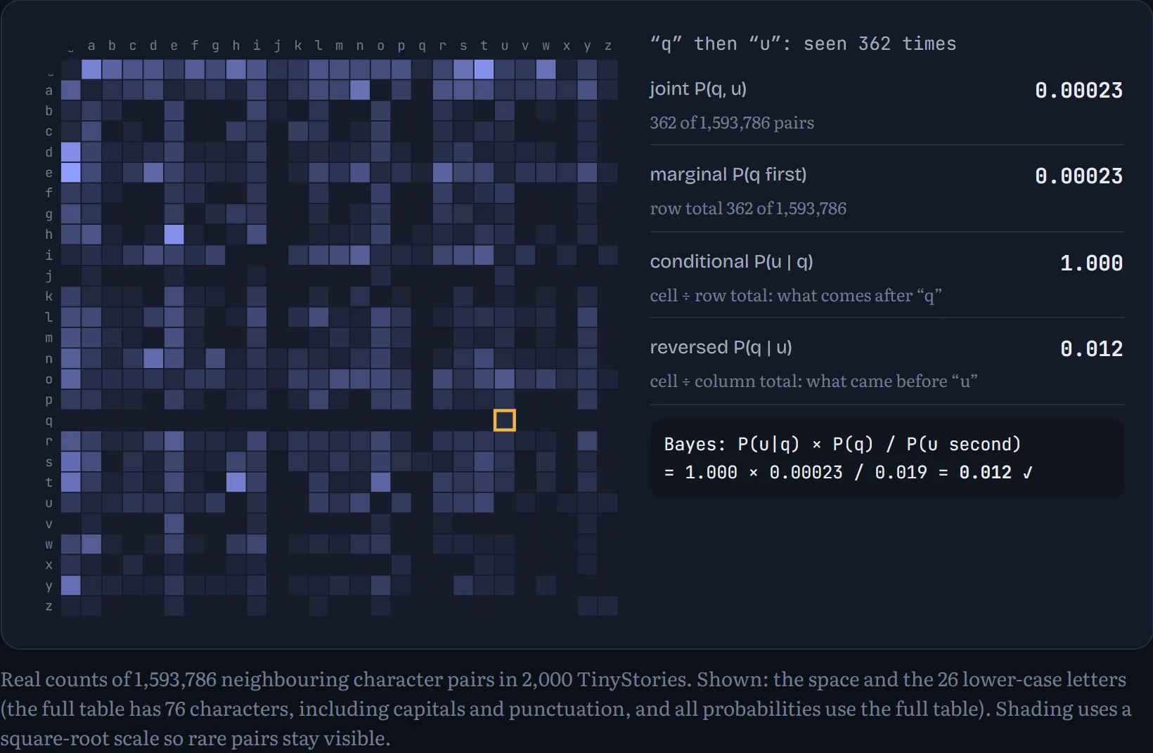
Bayes' rule turns a conditional around: P(a | b) = P(b | a) × P(a) / P(b). Read it with the q-u pair. After a q, a u is almost certain. But given a u, the character before it is very rarely a q, because u follows lots of letters and q is rare. The two conditionals measure different things, and confusing them is one of the most common reasoning errors there is, in medicine (“the test is 99% accurate, so a positive result means I'm 99% likely to be ill”) as much as in maths.
The probability of a whole sentence
How likely is a whole sentence? The chain rule of probability breaks it into steps: P(c₁, c₂, c₃, …) = P(c₁) × P(c₂ | c₁) × P(c₃ | c₁, c₂) × … Every language model, from your bigram to GPT, is a machine for estimating those conditional factors, one character or token at a time. A bigram model makes the simplifying bet that only the previous character matters, so each factor becomes P(cₜ | cₜ₋₁).
Multiply many numbers below 1 and you quickly get something too small for a computer to store, so in practice we add logarithms instead: log(x × y) = log x + log y. In the figure: a piece of text. Each character shows the bigram's probability for it given the one before; the total underneath is the log₂ probability of the whole string, compared with what a model that knows nothing (every one of the 76 characters equally likely) would give it.
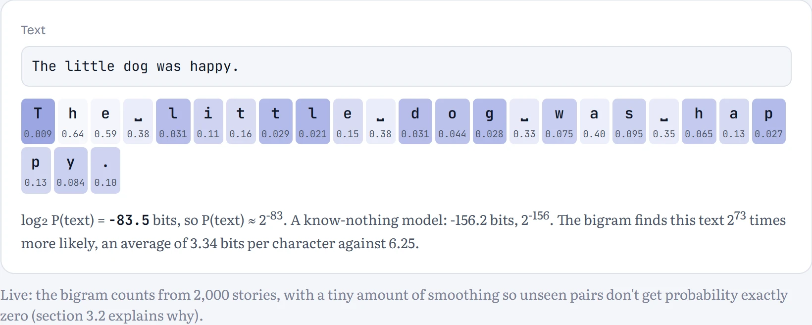
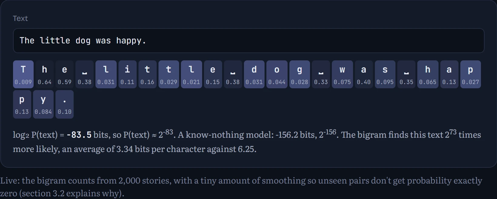
Predict first. Under this bigram model, which is more probable: “the cat sat” or “eht tac tas” (the same letters, each word reversed)?
- “the cat sat”, by a factor of thousands or more
- About the same: same letters
- “eht tac tas”
Answer. log₂ P(“the cat sat”) = -31.3 and log₂ P(“eht tac tas”) = -53.6, so the real phrase is about 2^22 ≈ 5,263,547 times more probable. Same letters, but the bigram cares about order: “th” and “he” are among the most common pairs in English, while “ht” and “eh” are rare. The chain rule multiplies those differences across every step.
Expectation and sampling
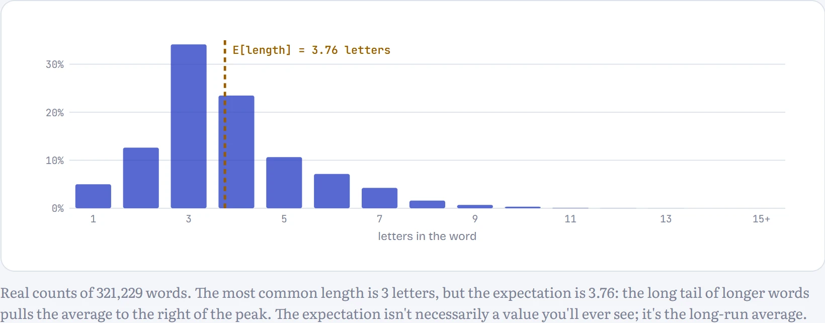
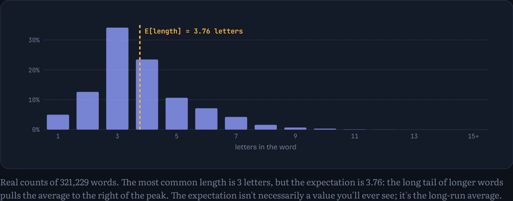
A distribution lists every possible outcome with its probability. The expectation (or expected value) is the probability-weighted average outcome: E[X] = Σ x · P(x). How to read the chart: the distribution of word lengths in the same 2,000 stories, where each bar is the share of words with that many letters; the marked line is the expectation.
Generating text means sampling: picking an outcome at random, so that each one comes up as often as its probability says. Computers do it with one uniform random number between 0 and 1. Stack the probabilities end to end into a bar of length 1, see where the random number lands, and output whatever owns that stretch. Likely characters own long stretches, so they're hit more often. In the figure: The top bar is the next-character distribution after the last character, the marker shows where the random number fell, and the text grows one sample at a time.
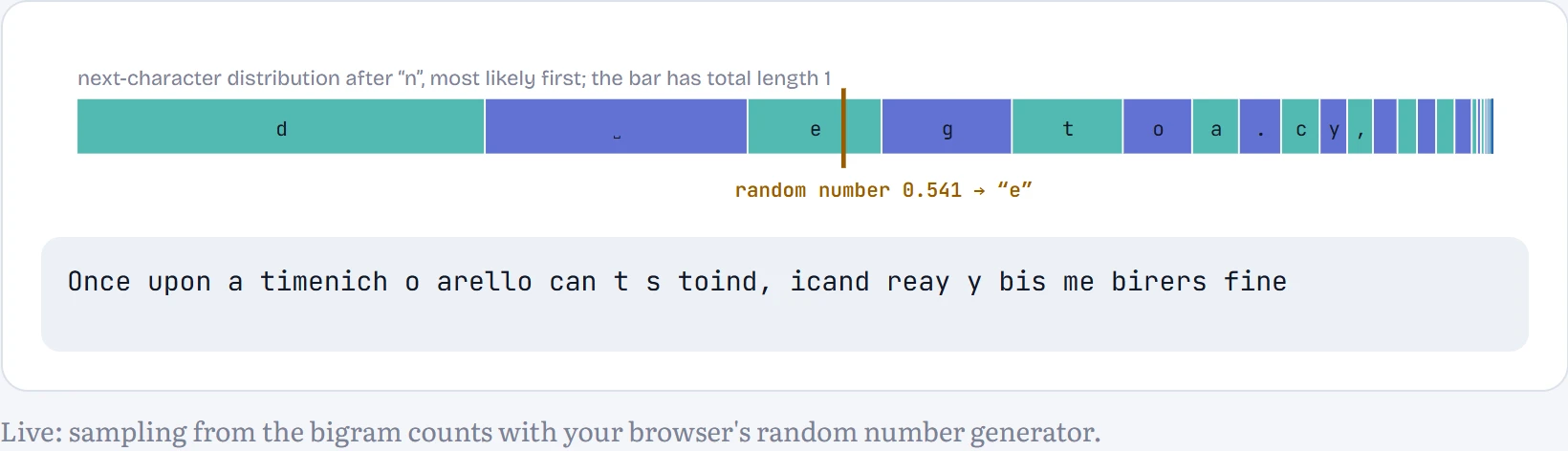
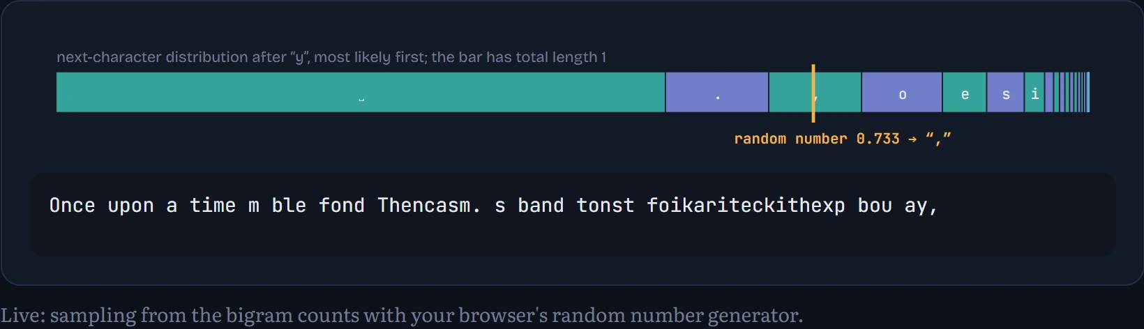
The output looks like English in texture and is nonsense in meaning, which is exactly what a model that only knows one character of context should produce. Everything that follows in this course is about estimating those conditional probabilities better, with more context.
Learning is estimation
Why is counting the right way to estimate the bigram's probabilities? Take one question: after a “t”, how often does an “h” come next? Call that unknown probability p. If we've seen n “t”s and k of them were followed by “h”, the probability of seeing exactly that data, for any guess of p, is proportional to pk(1 − p)n−k. That's the likelihood. The guess that makes the observed data most likely is the maximum likelihood estimate (MLE), and with a little calculus (set the derivative of the log-likelihood to zero) it comes out as p = k / n. Counting is maximum likelihood.
In the figure: the demo draws n random “t”s from the real stories and counts how many are followed by “h”. The chart shows the log-likelihood of every possible p (we use the log because it turns a product into a sum and has the same peak).
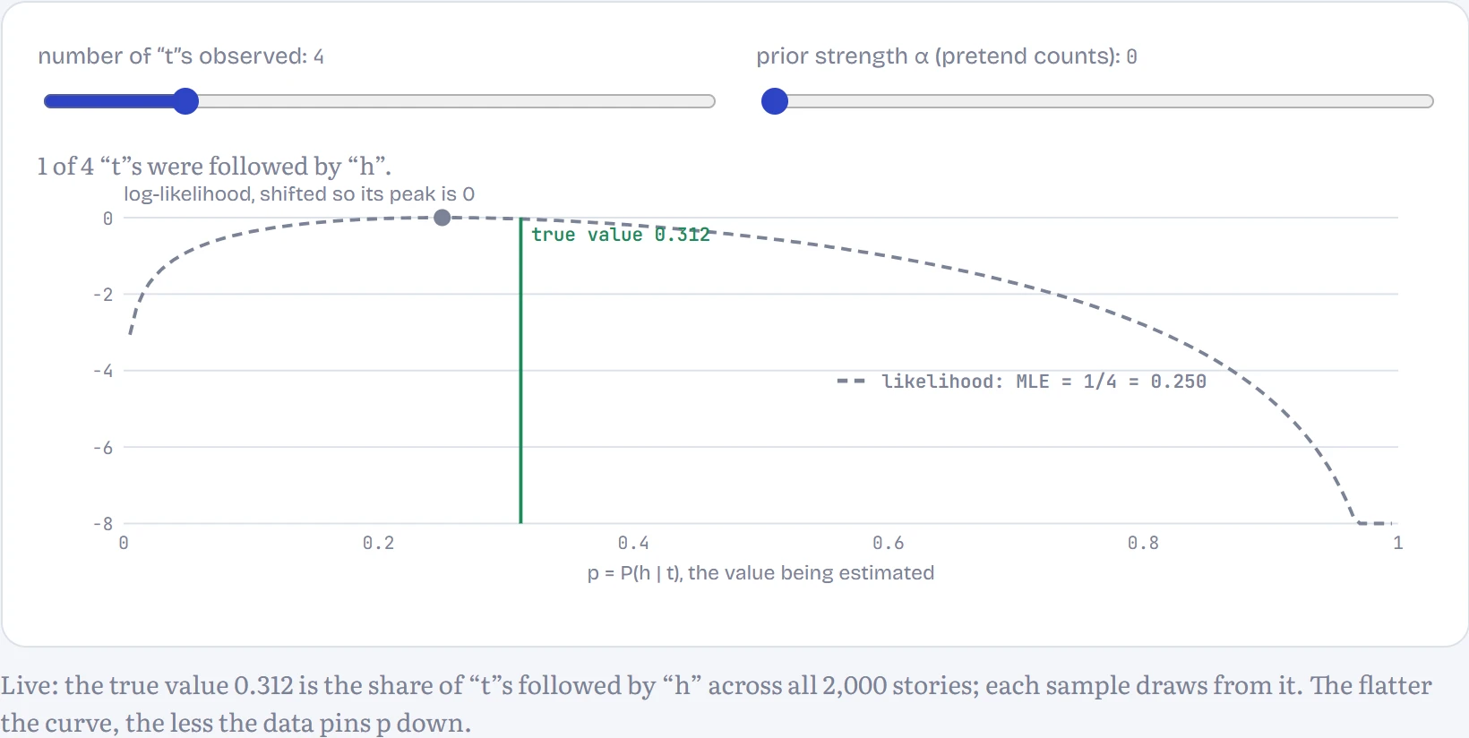
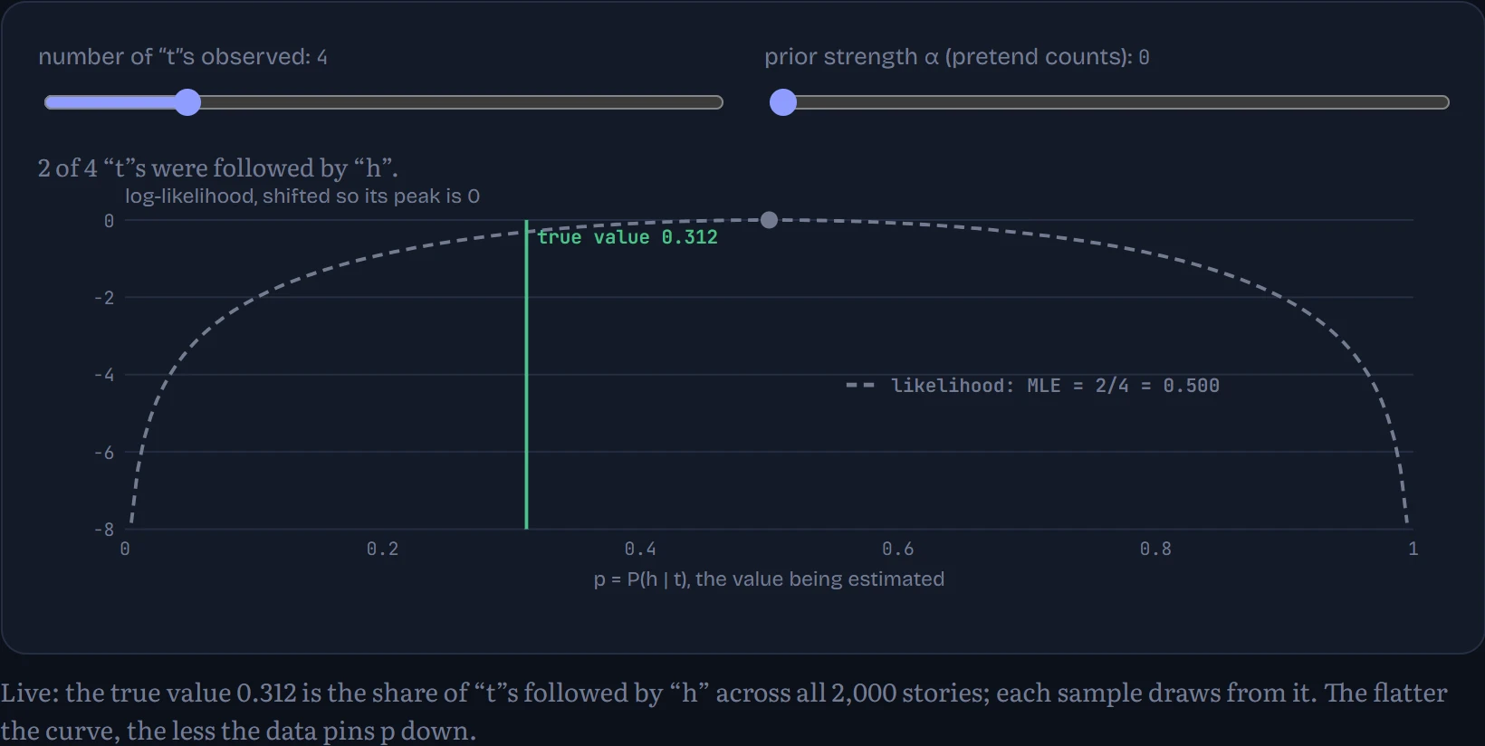
With 4 observations the estimate jumps around wildly, and if none of them happened to be followed by “h” the MLE says p = 0: “h never follows t”, which is false and, as we'll see, infinitely costly. The fix is to bring in a prior, a belief held before seeing the data, and find the most probable p given both. That's the maximum a posteriori (MAP) estimate. For counting, a simple prior is equivalent to adding α pretend observations of every outcome: p = (k + α) / (n + 2α) for a yes-or-no question, or (count + α) / (total + α × V) across V characters. That's add-α smoothing. In neural networks the same idea appears as weight decay, which is MAP with a prior that says weights are probably small.
How much prior is right depends on how much data you have and how many things you're estimating. I built character models that look back 0 to 5 characters (order 1 to 6, where order 2 is the bigram), trained on 200, 2,000 or 20,000 stories, and measured their quality on 400 held-out stories for a range of α. How to read the chart: bits per character on held-out text (lower is better; the next section explains the unit) against α; each line is one model order. Missing points at α = 0 mean pure counting assigned probability zero to something in the held-out text.
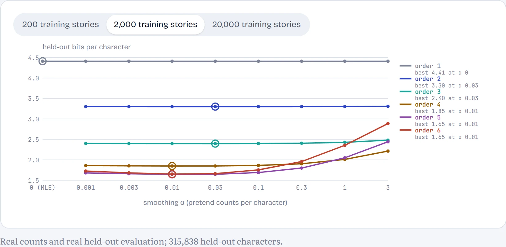
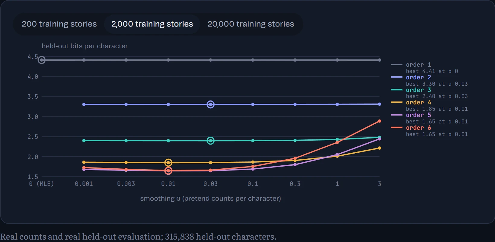
Three things to read off. First, pure counting (α = 0) fails outright for every model that uses context, at every data size: even trained on 20,000 stories, the bigram meets 7 held-out characters it calls impossible and the order-6 model 3,232, and one impossible event makes the average surprise infinite. (With only 200 stories, even plain character frequencies fail: 9 held-out characters never appeared in training at all.) A small prior fixes that, and the best α is small, around 0.01 to 0.03 pretend counts. Too much prior (α = 3) hurts the long-context models most: they have so many contexts, each seen only a few times, that the pretend counts swamp the real ones.
Second, the best amount of context depends on the data. With 200 stories the winner is order 4 (2.09 bits); longer contexts do worse because most of them were seen once or never. With 20,000 stories, order 6 wins (1.40 bits). Third, look at memorization: the order-6 model built from 200 stories scores 1.13 bits per character on its own training text and 2.43 on new text. Built from 20,000 stories the gap shrinks to 1.31 against 1.40. That's Chapter 4's overfitting, appearing in the simplest model there is. Counting can't share what it learns between similar contexts, and that limitation is why we move to neural networks.
Surprise, entropy and cross-entropy
How surprised should you be by an outcome with probability p? Claude Shannon's answer (1948) is −log₂ p bits. A fair coin flip is 1 bit of surprise; a 1-in-8 event is 3 bits; a certain event is 0. The unit is the bit because it's literally the number of yes-or-no questions it would take to pin the outcome down. The average surprise of a distribution, weighted by how often each outcome happens, is its entropy: H(p) = −Σ p(x) log₂ p(x). It measures how unpredictable the thing is.
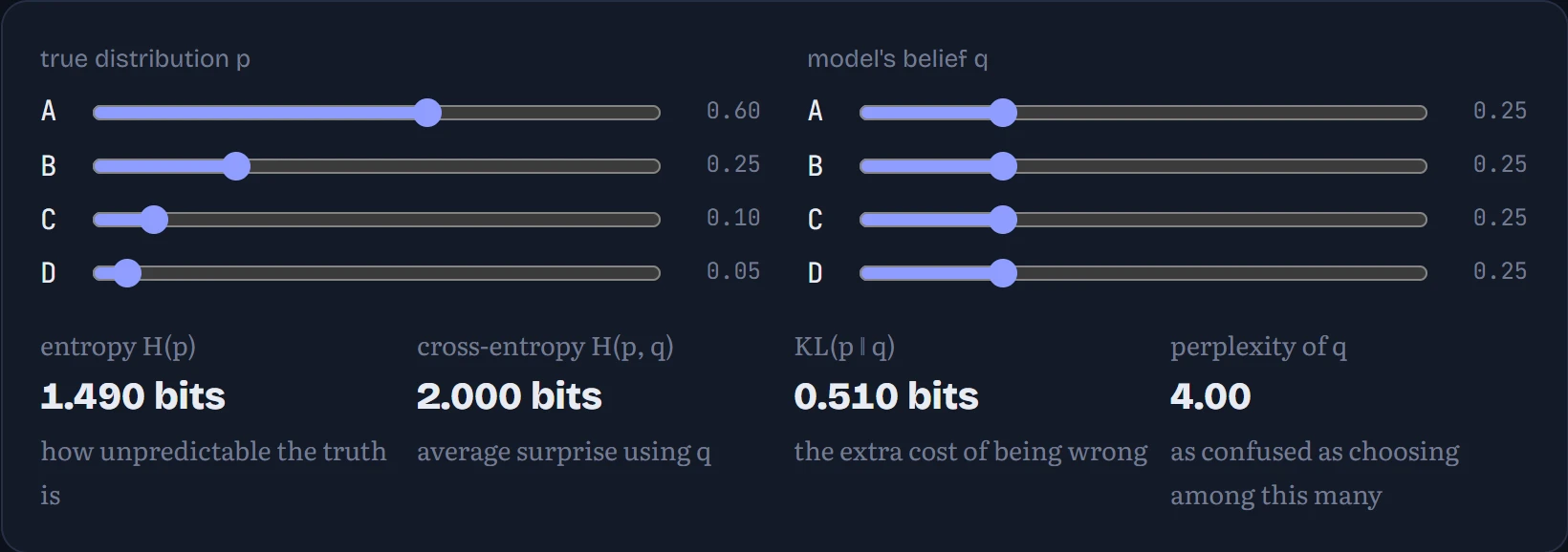
Now suppose the truth is p but your model believes q. You'll be surprised by −log₂ q(x) each time, and averaged over the true frequencies that's the cross-entropy H(p, q) = −Σ p(x) log₂ q(x). It can never be lower than H(p); the gap, H(p, q) − H(p), is the KL divergence, the extra bits you pay for believing the wrong thing. Training a language model with cross-entropy loss means exactly this: making its q as close to the text's true p as it can. In the figure: the true distribution (top) and the model's belief (bottom) over four outcomes.
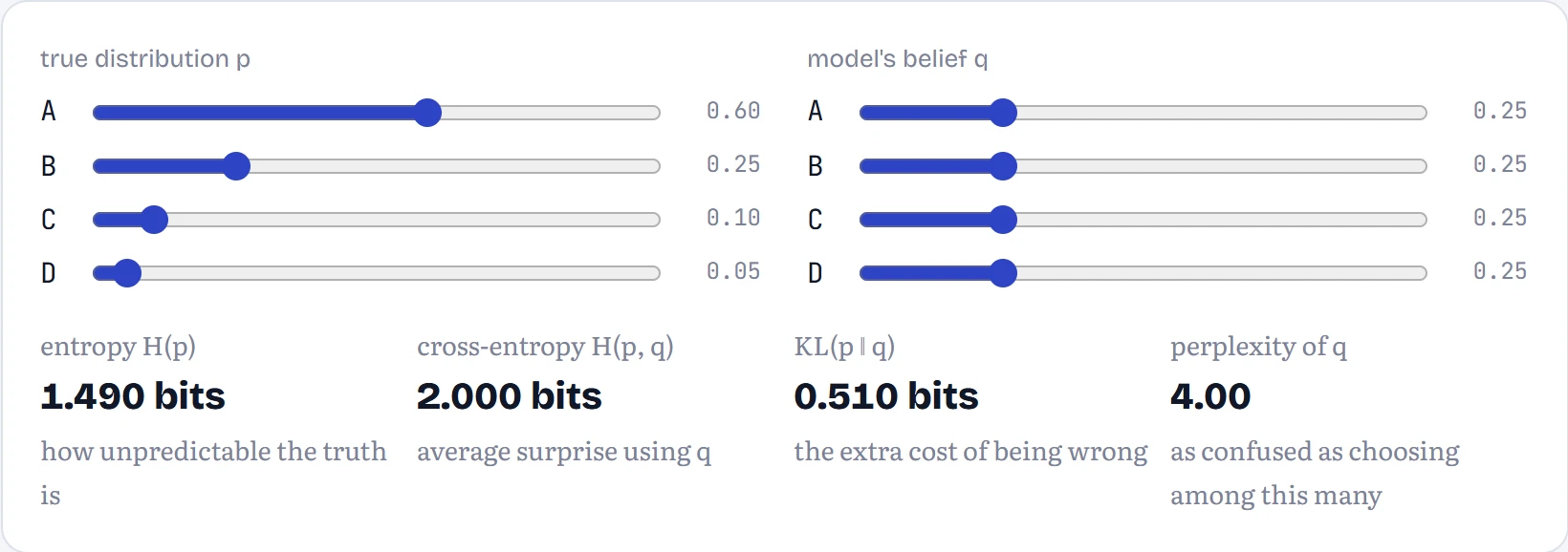
Two more names you'll see everywhere. Perplexity is 2 to the power of the cross-entropy in bits: a model with 2 bits per character is “as confused as if it were choosing uniformly among 4 characters”. And language models usually report loss in nats, the same thing with natural logs: divide by ln 2 ≈ 0.693 to get bits.
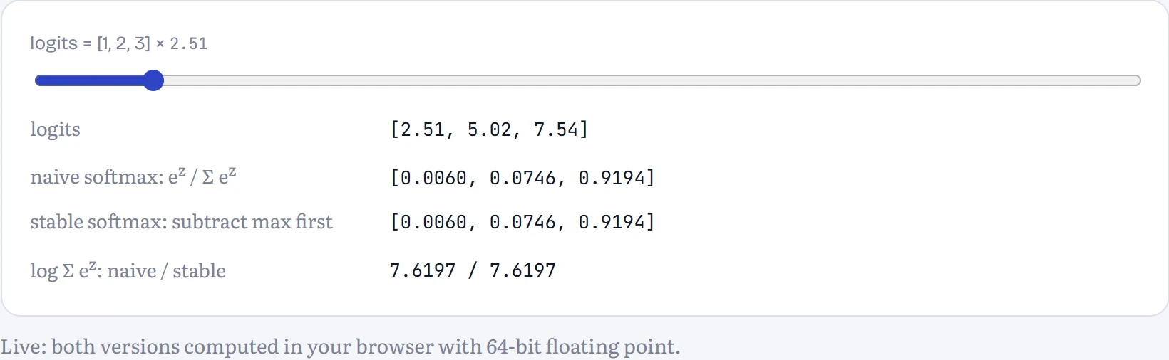
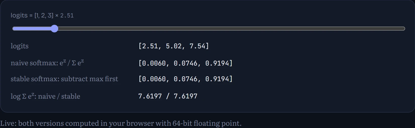
One practical detail. A model produces raw scores (logits) and turns them into probabilities with the softmax, ezᵢ / Σⱼ ezⱼ. Computed naively, e1000 overflows to infinity and the answer becomes NaN (not a number). The fix is to subtract the largest logit first, which doesn't change the result (it cancels between top and bottom) but keeps every exponent at 0 or below. The same trick computes log Σ ezⱼ, the log-sum-exp at the heart of cross-entropy. In the figure: as the logits are scaled up, the naive version breaks while the stable one carries on.
Prediction is compression
Here's the idea that makes “bits per character” more than a metaphor. Shannon showed that a model which gives an outcome probability p can be used to store it in −log₂ p bits (a technique called arithmetic coding gets within a hair of that). So a model's cross-entropy on some text, in bits per character, is exactly the size it could compress that text to. A better predictor is a better compressor, and the other way round.
That lets us put language models and ordinary file compressors on one scale. How to read the chart: bits needed per character of the 400 held-out stories (lower is better). Plain ASCII uses 8. The compressors (gzip, bz2, lzma, as built into Python) see only the held-out text itself; the models were trained on separate stories.
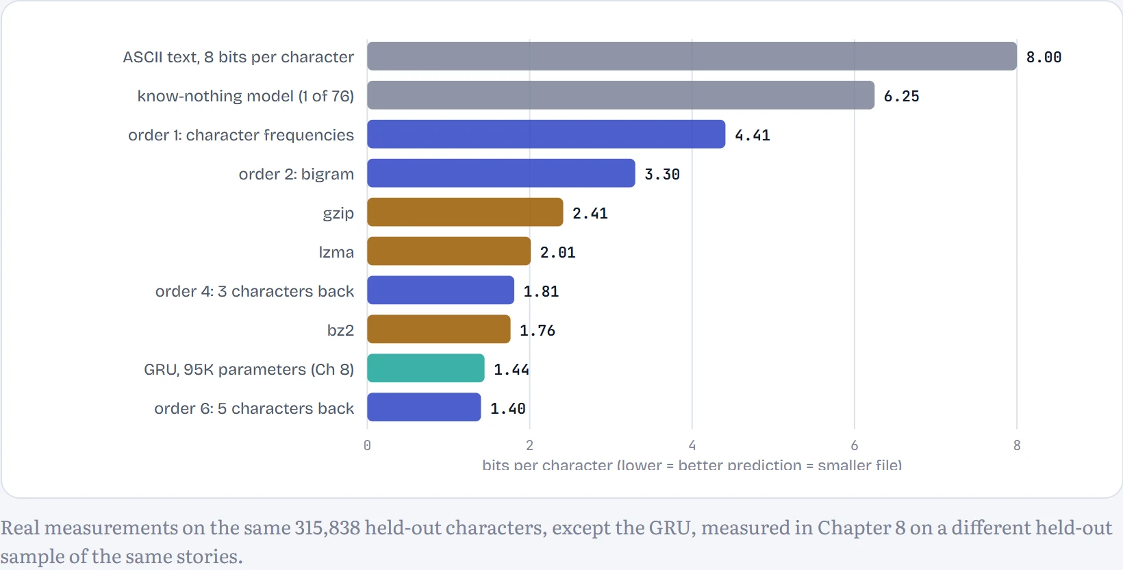
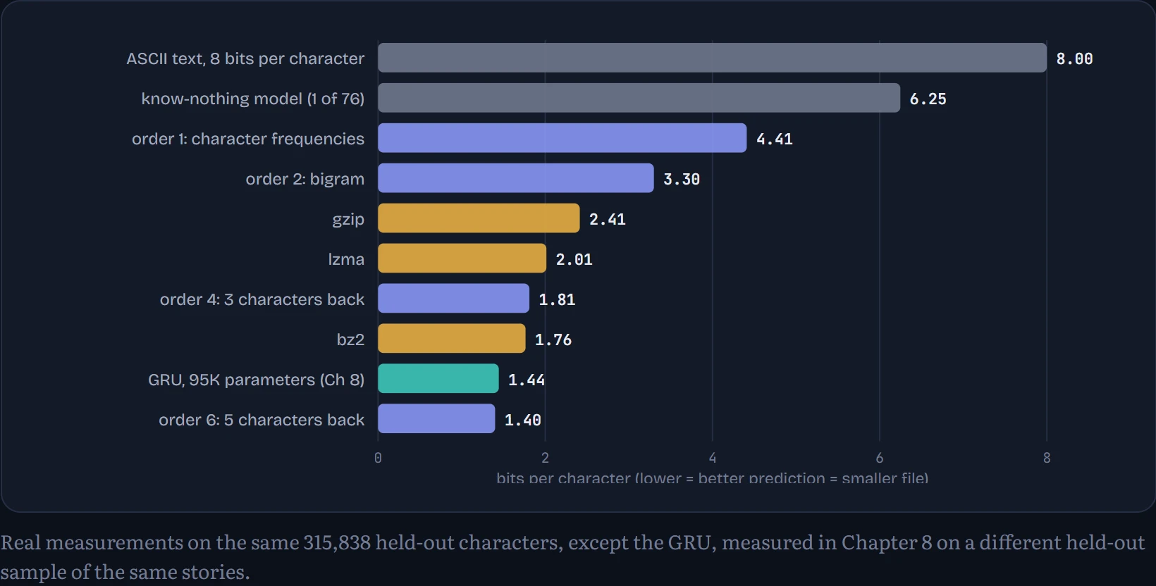
How to read the chart: blue bars are counting models trained on 20,000 other stories, amber bars are general-purpose compressors, teal is the small neural network from Chapter 8. Knowing nothing costs 6.25 bits per character (log₂ of 76). Just knowing how common each character is gets you to 4.41, which is the entropy of the character distribution. The bigram reaches 3.30, already beating gzip (2.41). The order-6 model, at 1.40 bits, beats bz2 (1.76), the best of the three compressors, by a wide margin.
That's not quite a fair fight: the compressors start from nothing and learn as they go through 316,000 characters, while the n-gram brought knowledge from 20,000 other stories (and storing it would take far more space than the text). It makes the point all the same: compression and prediction are the same problem, and what you know in advance is worth bits. One surprise: the order-6 count table (1.40) slightly beats the GRU from Chapter 8 (1.44). The GRU saw fewer characters in training (about 12 million against 16 million) with only 95,000 parameters, while the count table stores millions of contexts. Bigger neural models trained longer win easily, as Chapter 7's mini_lm and Chapter 9's mini-GPT show, but size and data matter as much as architecture. This is also why language-model researchers say a model that predicts text well must have “compressed” something real about the world that produced it.
Continue the lesson
The whole lesson, with its drawings and its questions. 7 more sections after the ones above.