
Backpropagation: a reverse-mode autograd engine, nonlinearities, SGD, momentum and Adam
A neuron weighs its inputs, adds a bias and squashes the total, so one neuron draws one line. Stacking neurons with a non-linear activation lets a network bend. Backpropagation runs the network forward, then sends gradients backward through the graph, and an optimizer such as SGD, momentum or Adam decides what to do with them.
What this page answers
Can a single neuron solve XOR?
No. The two classes sit on opposite diagonals, so no single straight line separates them. A network needs a hidden layer with a non-linear activation to bend the boundary. Read it in “One neuron draws one line”
How does an autograd engine compute gradients?
Each operation stores its local derivative on the way forward. backward() then visits the nodes in reverse topological order and accumulates gradients with +=, so a value used twice receives both contributions: the multivariable chain rule. Read it in “The engine: two rules and a sort”
One neuron draws one line
Strip away the biology metaphors. A “neuron” takes some numbers, multiplies each by a weight, adds them up with a bias, and passes the total through a squashing function. With two inputs, w₁x + w₂y + b is zero along a straight line, positive on one side and negative on the other. The squashing function turns “how far, and which side” into an output between, say, 0 and 1.
So one neuron is a line-drawer.
Think of deciding whether to take an umbrella. You look at two things, how cloudy it is and what the forecast says, and you trust them differently. Each weight is how much you trust one input, and its sign says which way it pushes. The bias is your general mood: a cautious person takes the umbrella with less evidence. Add it all up; if the total is above zero, take the umbrella. The squashing function just turns that hard yes/no into a smooth “how sure”, between 0 and 1.
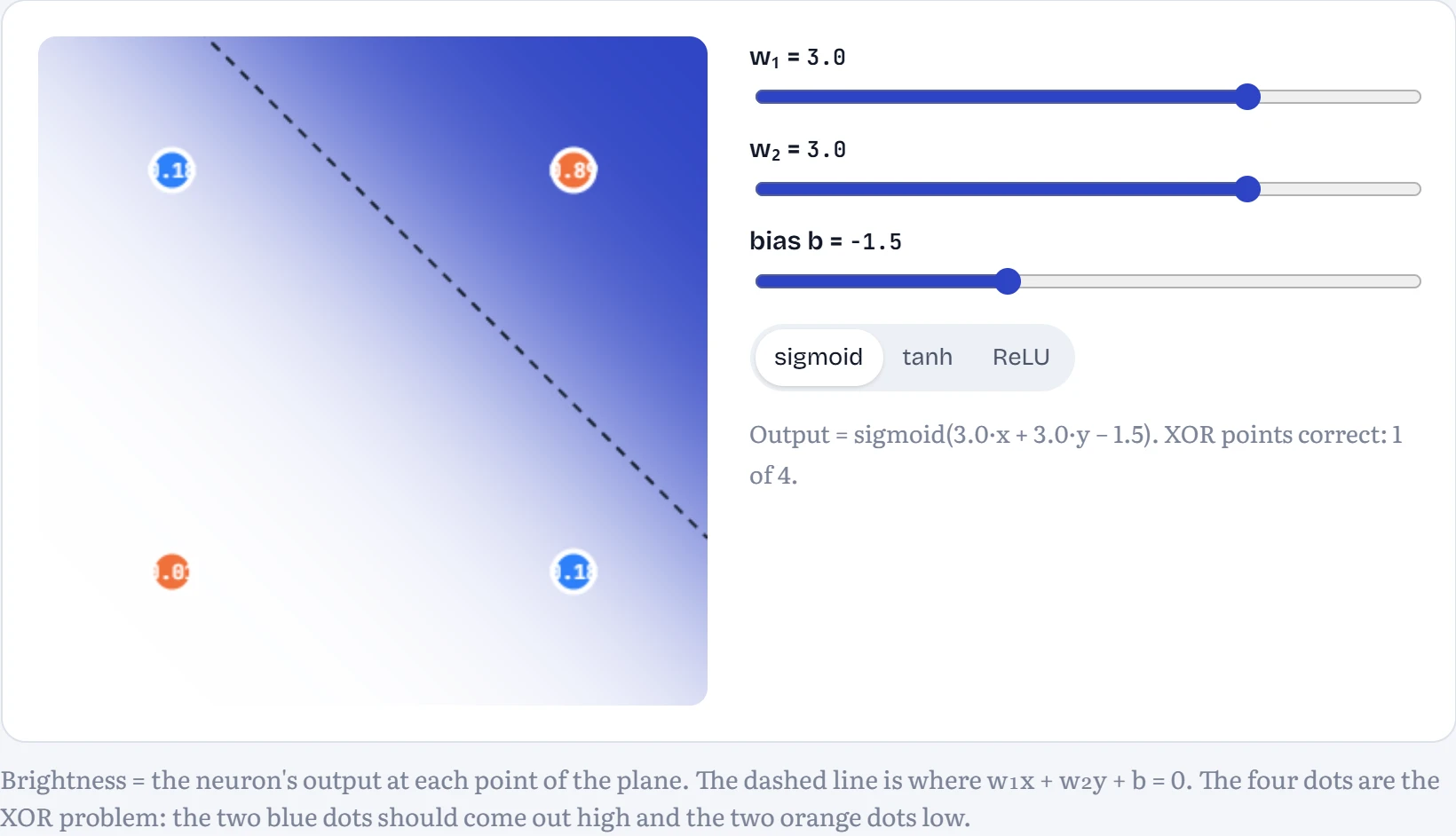
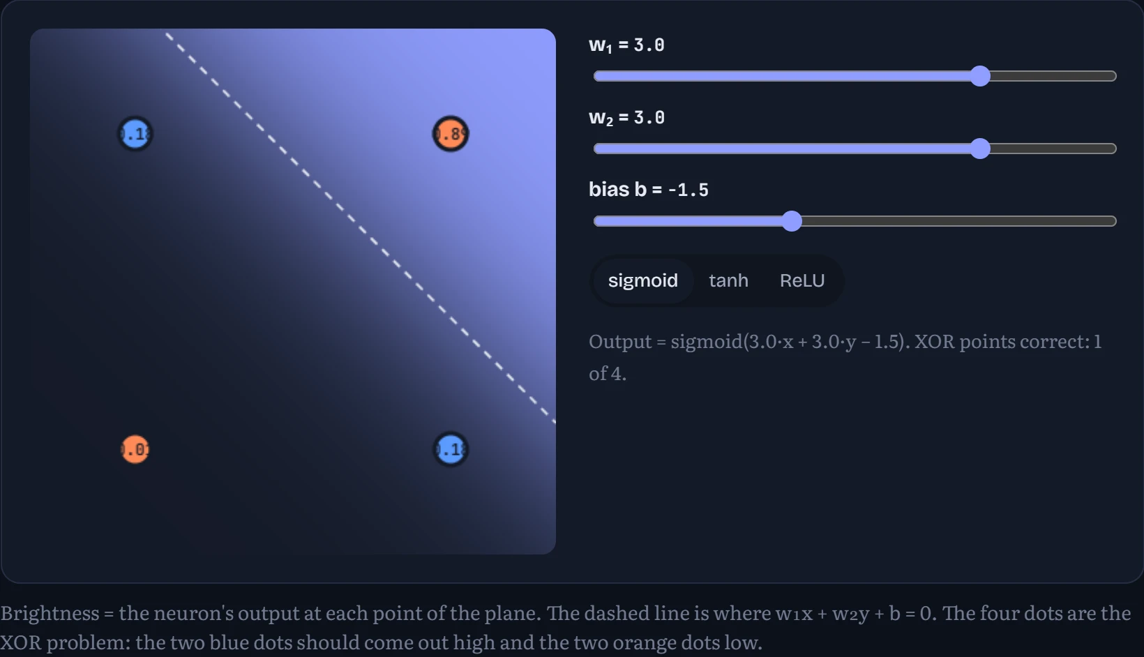
Predict first. Are there weights where both blue dots light up and both orange dots stay dark? Can one neuron do it?
- Yes, with the right weights
- No, never
Answer. Never. The blue dots sit on one diagonal and the orange dots on the other, so no single straight line puts both blues on one side and both oranges on the other. This exact limitation, shown formally by Minsky and Papert in 1969, helped stall neural network research for over a decade. The fix is embarrassingly simple: use two neurons to draw two lines, and a third to combine them.
In the playground at the top of the lesson: XOR, one hidden layer, width 2. In principle two neurons are enough. In practice, from this starting point, training gets stuck at about 86% accuracy and stays there: a local minimum, a real hazard of small networks. With width 4 it solves the problem in a few hundred steps. Spare neurons make the loss landscape friendlier, which is part of why large networks are often easier to train than small ones.
Why the network must bend
If neurons draw lines, can't we stack lots of them and skip the squashing? Here's why not, in four lines of arithmetic. A layer without an activation computes W₁x. Stack a second one and you get W₂(W₁x). But matrix multiplication is associative, so that's (W₂W₁)x: a single matrix. A hundred linear layers collapse into one linear layer, and one linear layer can only draw one straight boundary.
With no activation at all (linear), trained on the spiral, adding layers or widening them does not help. The best it can ever do is a single straight cut through the data. With tanh, it curls around the arms.
Each line is one neuron's decision boundary. The network's curved final boundary is built by bending, combining and re-bending those straight pieces in later layers. That's the whole trick, and it's why ReLU, which just zeroes out negatives, is enough: it puts one kink in each neuron, and enough kinks make any shape.
Which bend? ReLU, GELU and friends
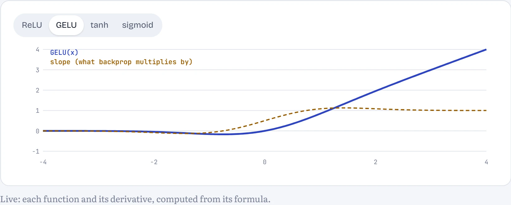
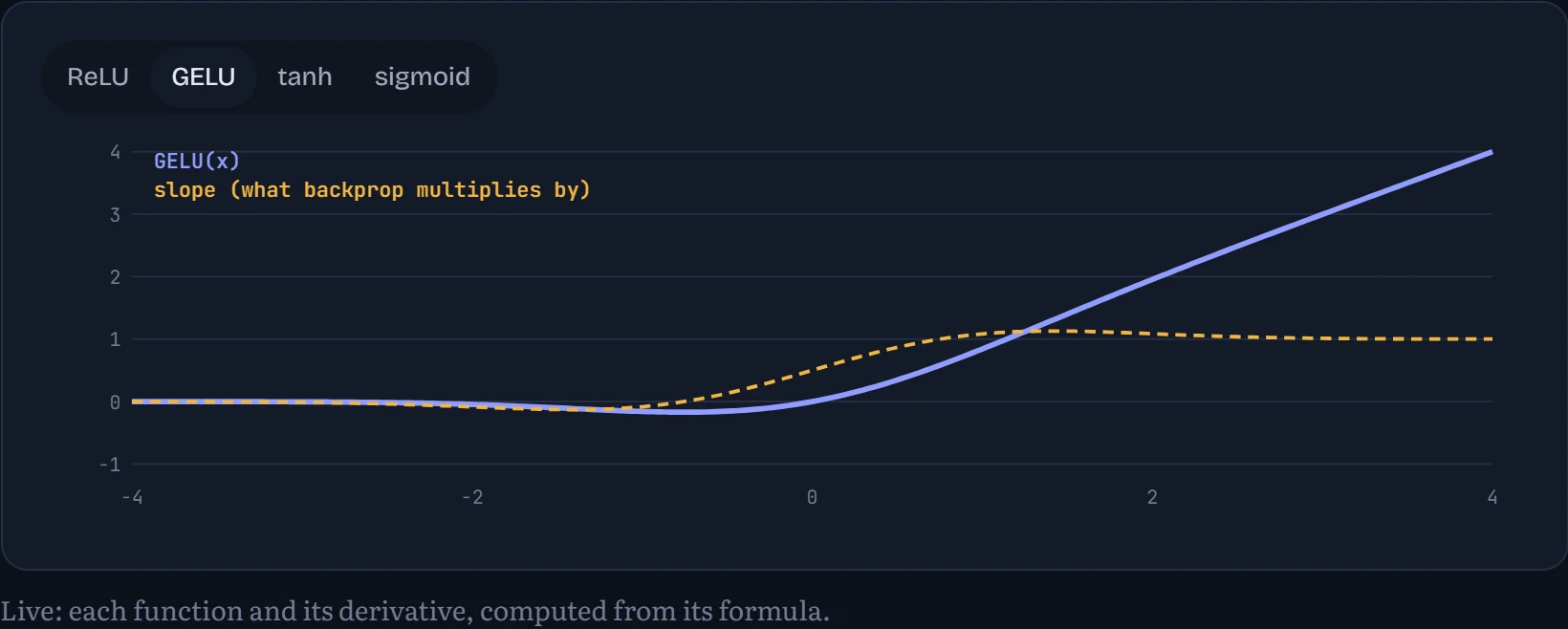
Any nonlinearity breaks the collapse, but they don't train equally well. Sigmoid squashes everything into 0 to 1 and tanh into −1 to 1; both go flat at the ends, so their slope (the number backprop multiplies by) is nearly zero for large inputs. ReLU, max(0, x), never goes flat for positive inputs, which is a big reason deep networks became trainable around 2010. GELU, used in GPT and almost every Transformer, is a smooth ReLU: it lets small negative values through a little instead of cutting them off sharply. In the figure: each function's shape (solid) and its slope (dashed).
Does the choice matter in practice? I trained the same MNIST network with each function, for two epochs with Adam, once shallow (2 hidden layers) and once deep (8 hidden layers). How to read the table: test accuracy on the 10,000 test digits.
| Activation | 2 hidden layers | 8 hidden layers |
|---|---|---|
| ReLU | 96.2% | 96.0% |
| GELU | 96.4% | 95.8% |
| tanh | 96.5% | 95.9% |
| sigmoid | 94.9% | 48.6% |
| none (linear) | 92.0% | 89.8% |
In the shallow network every real nonlinearity does well: ReLU 96.2%, GELU 96.4%, tanh 96.5%, sigmoid 94.9%, against 92.0% with no activation at all, which is just a linear classifier however many layers it has. Depth separates them. With 8 hidden layers, sigmoid falls to 48.6%: its slope is at most 0.25, so every layer shrinks the gradient by at least four times, the vanishing-gradient problem from the deep-network section below. ReLU does best (96.0%), with GELU 95.8%, tanh 95.9%. GELU's small advantages in large Transformers come from its smoothness helping optimization at scale; on a network this size it's essentially a tie with ReLU.
PRECISION NOTE. The universal approximation theorem says one hidden layer with enough units can approximate any continuous function on a bounded region as closely as you like. It says nothing about how many units that takes, or whether gradient descent will find the weights. In practice, depth gets there with far fewer parameters, which is why networks are deep rather than just wide.
Forward, then backward, on a graph you can check by hand
Training needs one thing: for every weight, how much would the loss change if I nudged it? That's the gradient. Here's a single neuron, o = tanh(x₁w₁ + x₂w₂ + b), written as a graph of tiny operations. It is stepped through below: first the values flow forward, then the gradients flow back. But first, what exactly is a gradient?
A gradient answers one question for each number in the graph: “if I nudged you up a tiny bit, how much would the final output move, and which way?” A gradient of 0.5 means the output moves half as much as the nudge; −1.5 means it moves one and a half times as much, in the opposite direction; 0 means you don't matter right now.
The chain rule is just gears. If gear A turns gear B twice as fast, and B turns C three times as fast, then A turns C six times as fast. Each node in the graph knows only its own “gear ratio” (its local derivative), and backpropagation multiplies the ratios along the path from the output back to each input.
How to read the graph: each box is one small calculation, and the arrows show which results feed into which. The top line of a box is its value; the bottom line, in colour, is its gradient. The steps walk forward through the values; in the lesson, a backward pass then fills in the gradients from right to left.
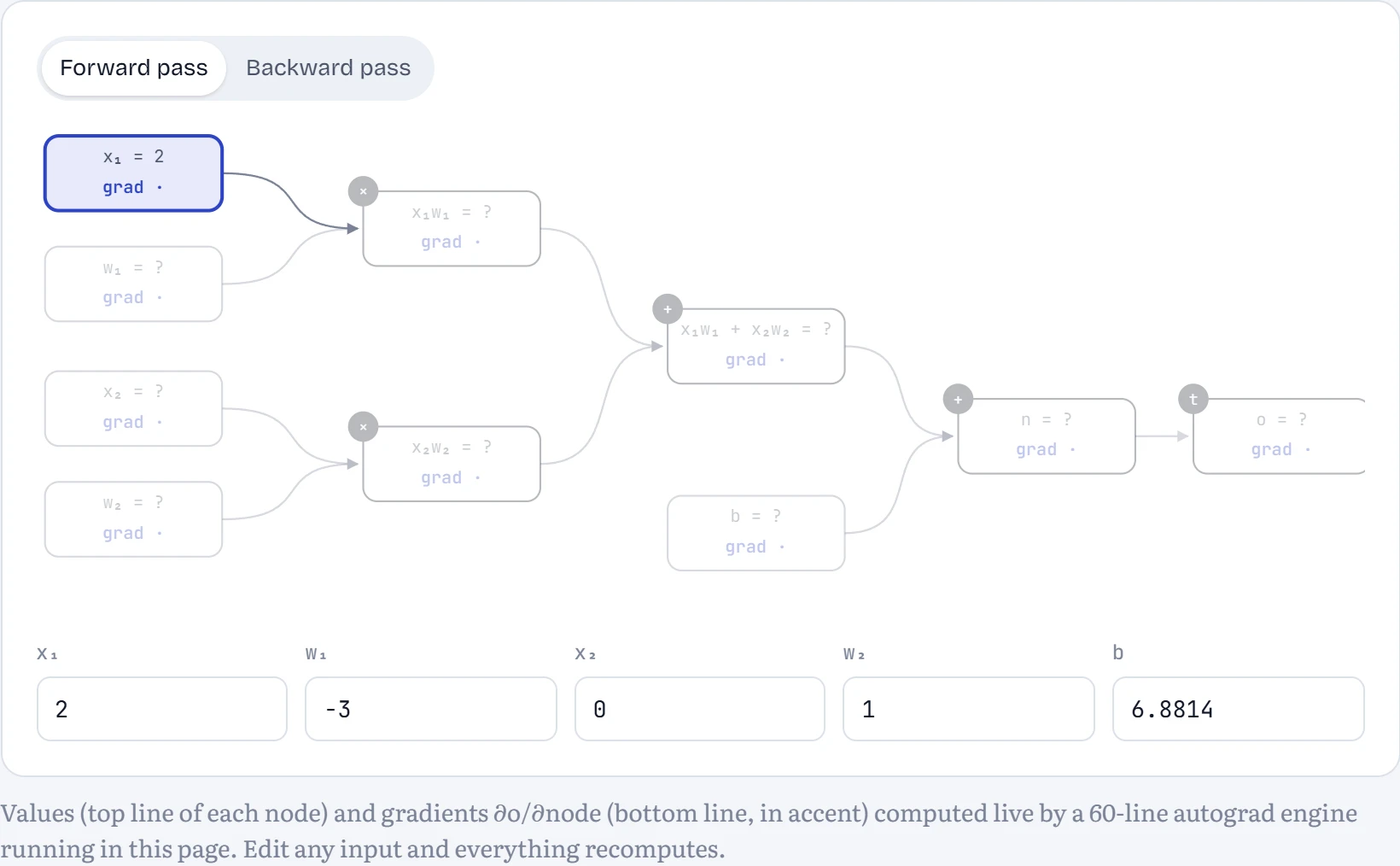
Step 1 of 10 Forward · Inputs and weights are just numbers to start with. No gradients yet.
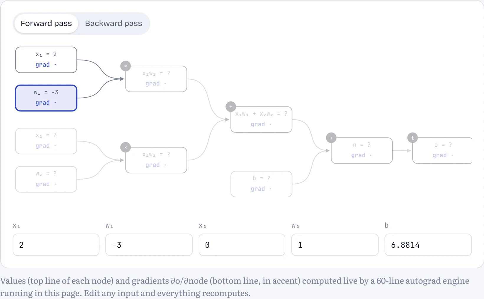
Step 2 of 10 Forward · Every leaf holds a value.
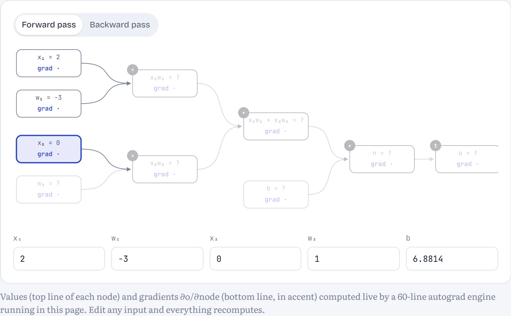
Step 3 of 10 Forward · x₂ is 0 here. Keep an eye on what that does later.
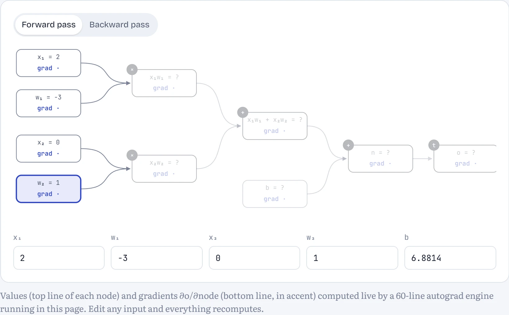
Step 4 of 10 Forward · Last weight.
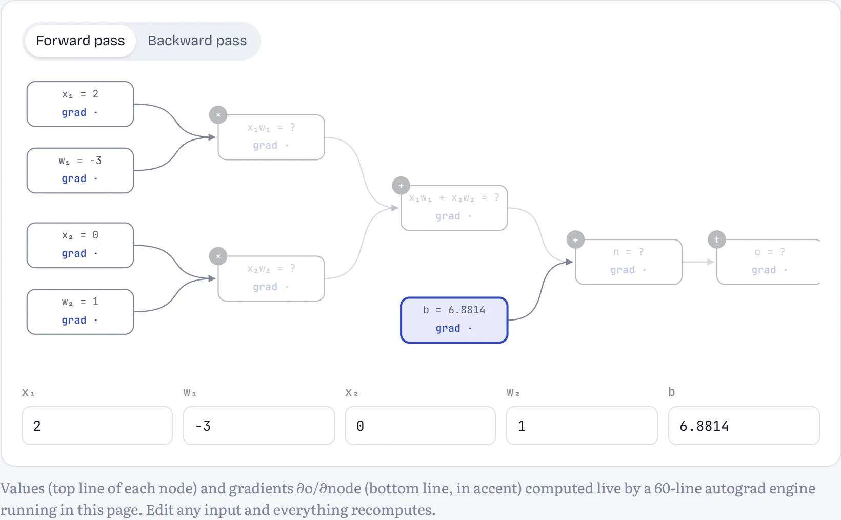
Step 5 of 10 Forward · The bias.
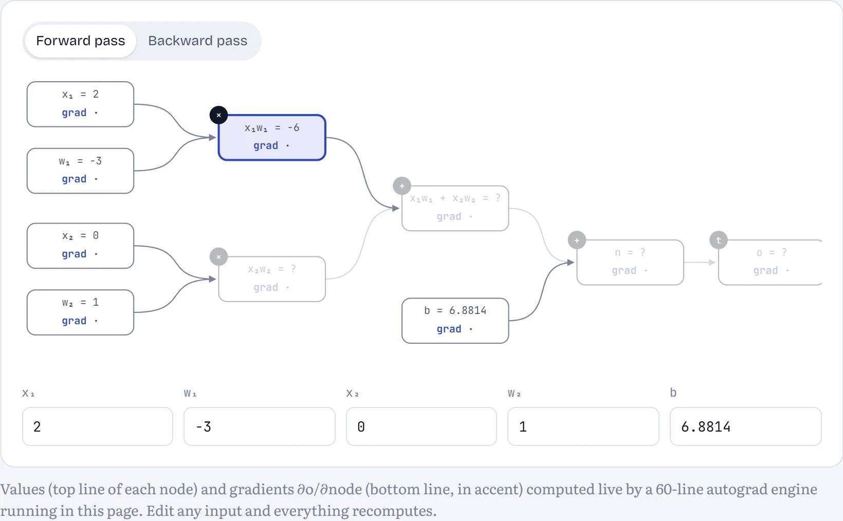
Step 6 of 10 Forward · “×” node: 2 × -3 = -6.0000.
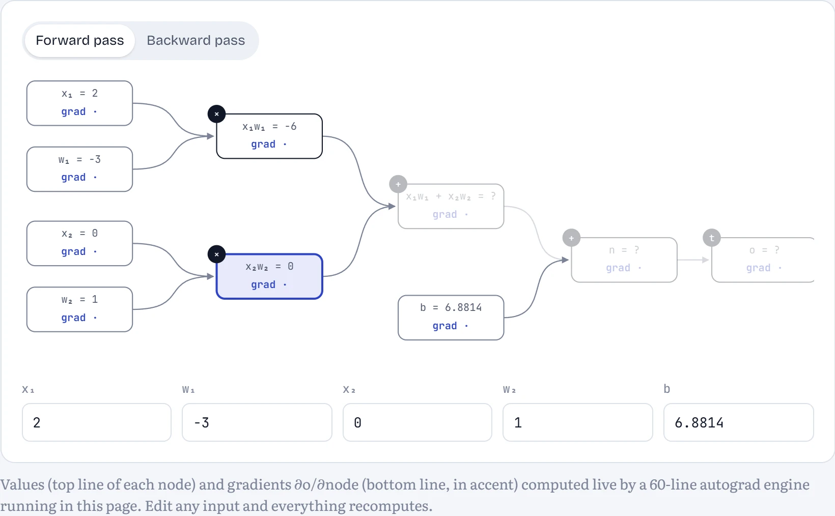
Step 7 of 10 Forward · 0 × 1 = 0.0000.
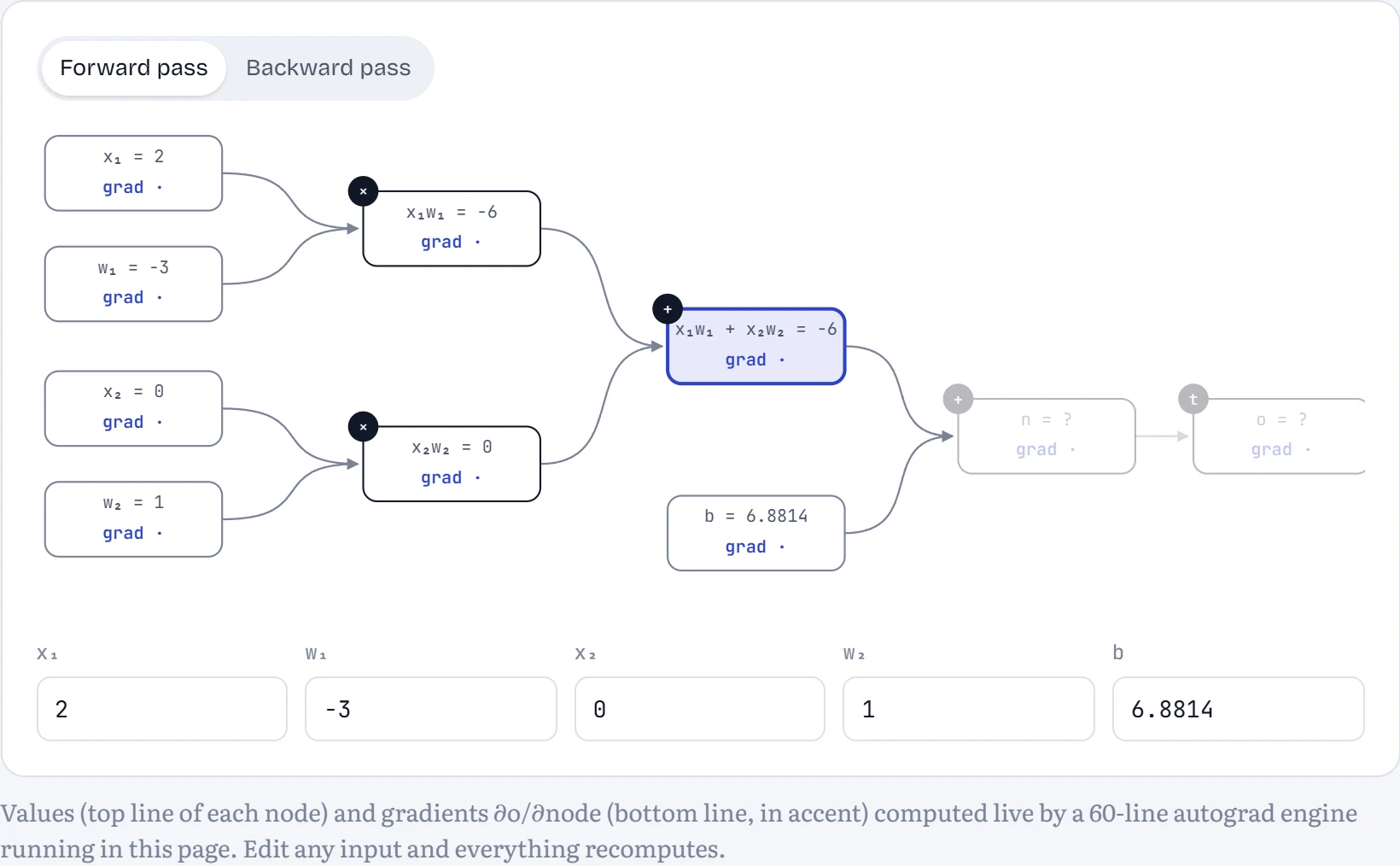
Step 8 of 10 Forward · “+” node: -6.0000.
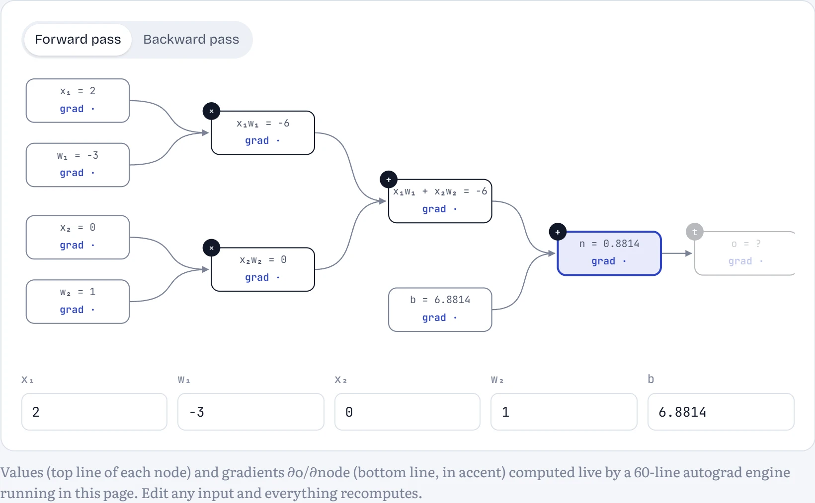
Step 9 of 10 Forward · Add the bias: n = 0.8814.
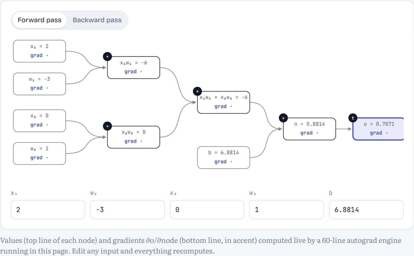
Step 10 of 10 Forward · Squash: o = tanh(n) = 0.7071. Forward pass done.
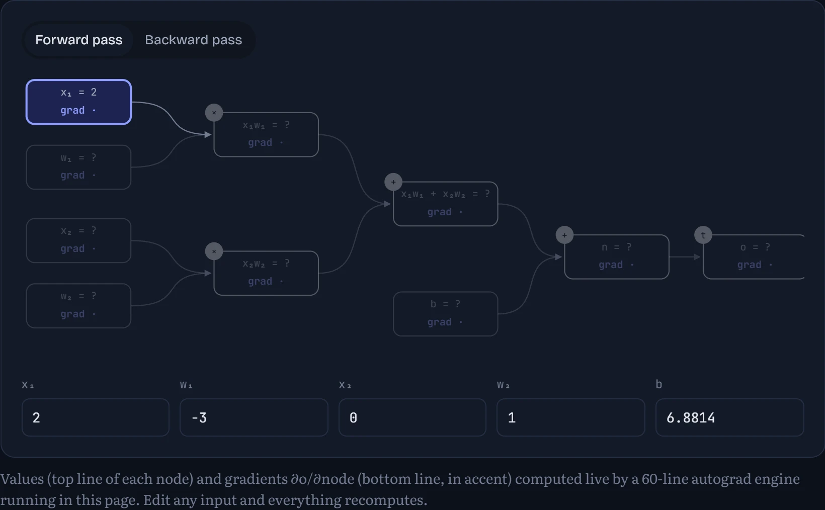
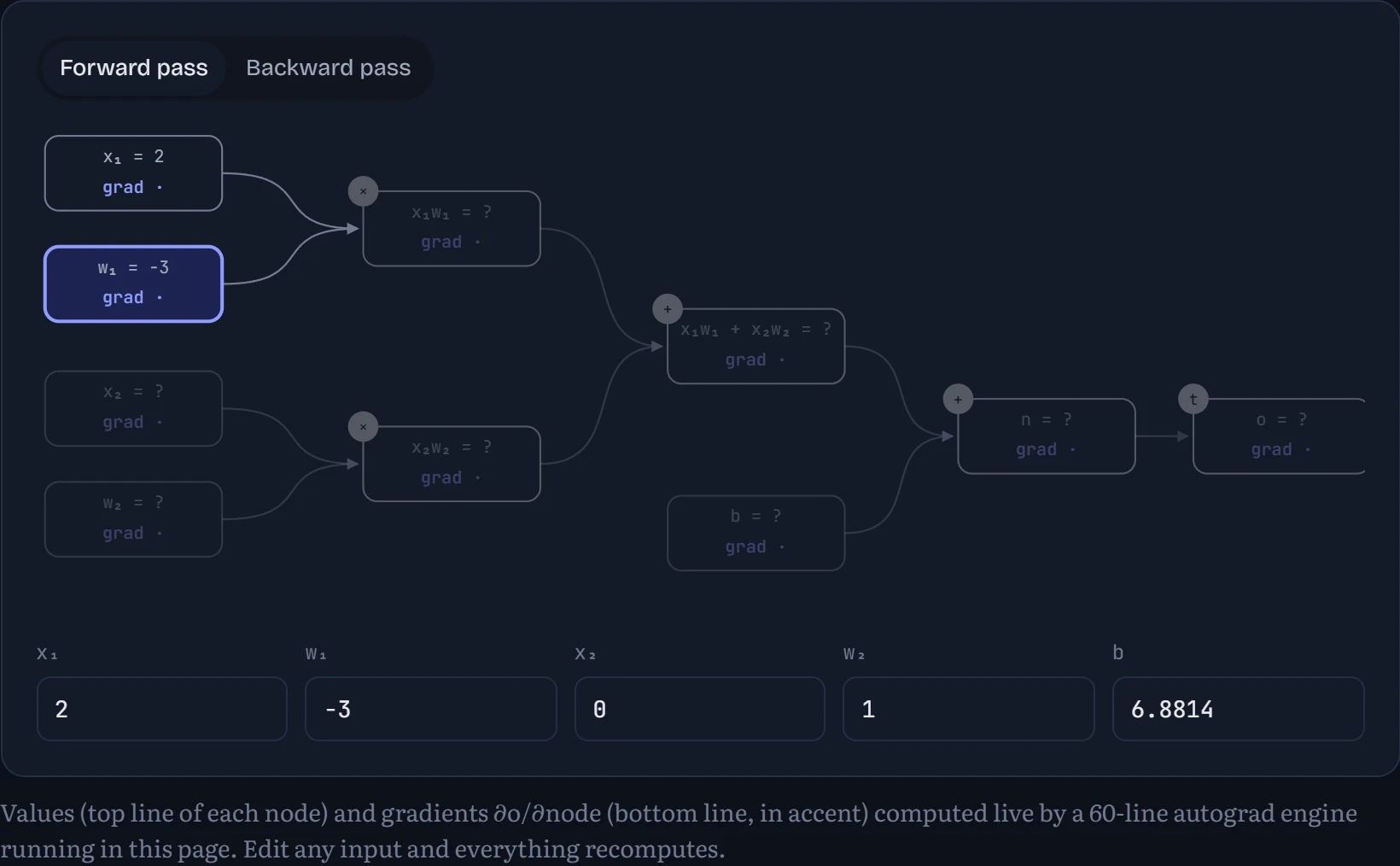
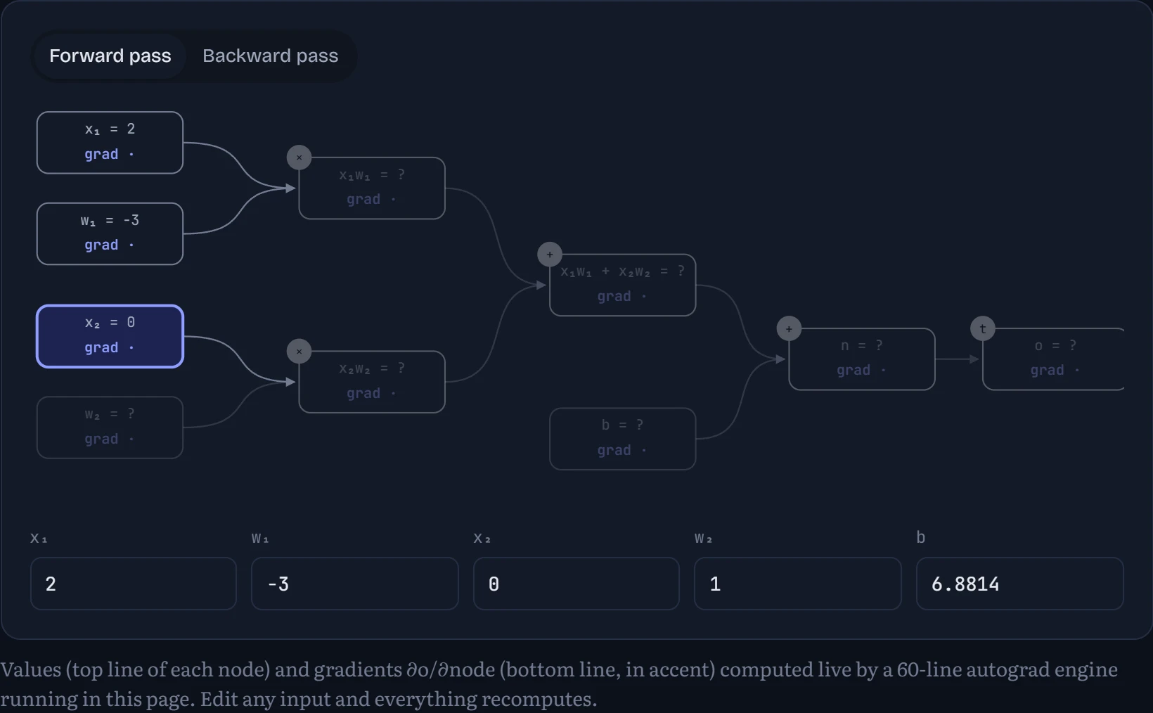
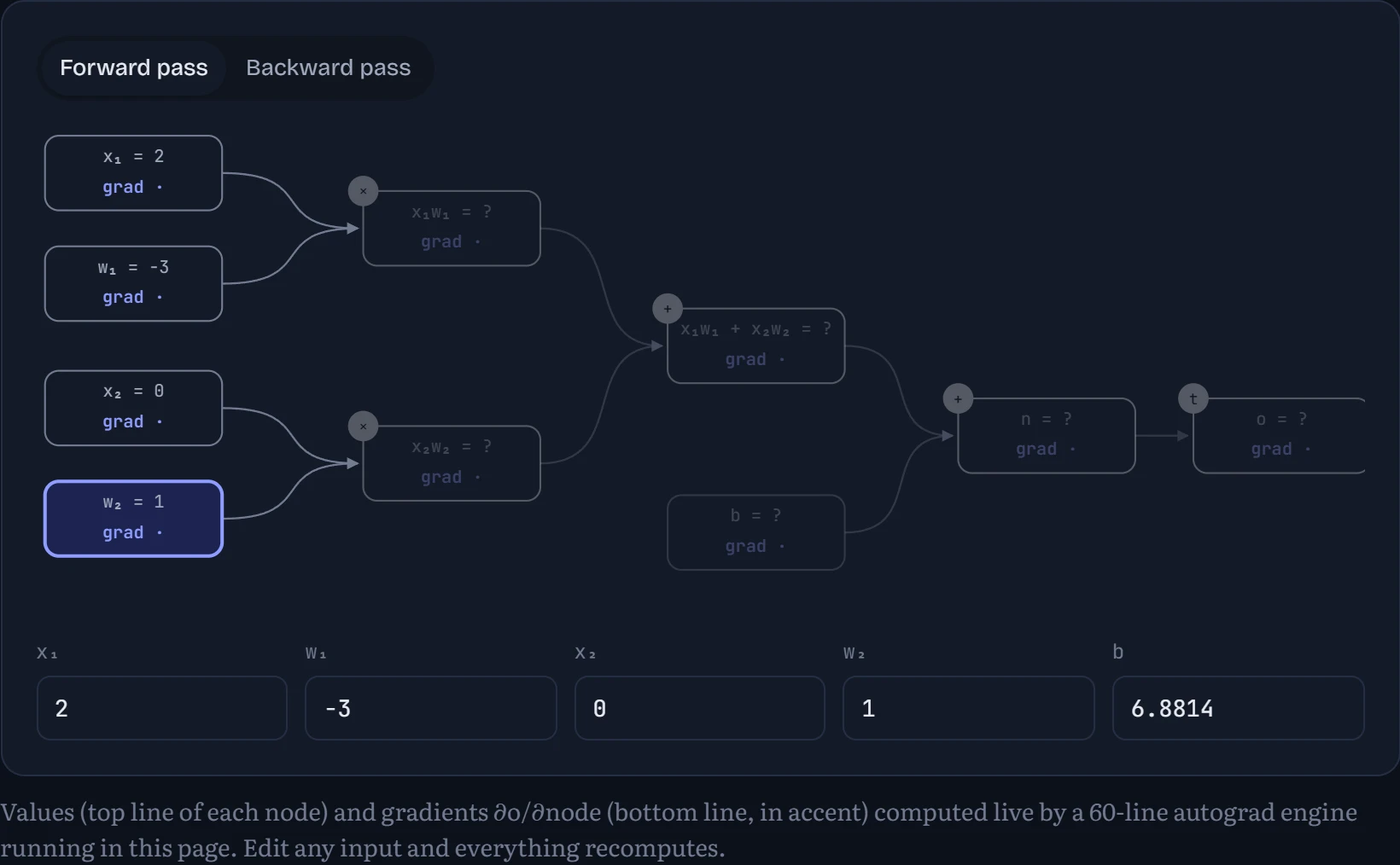
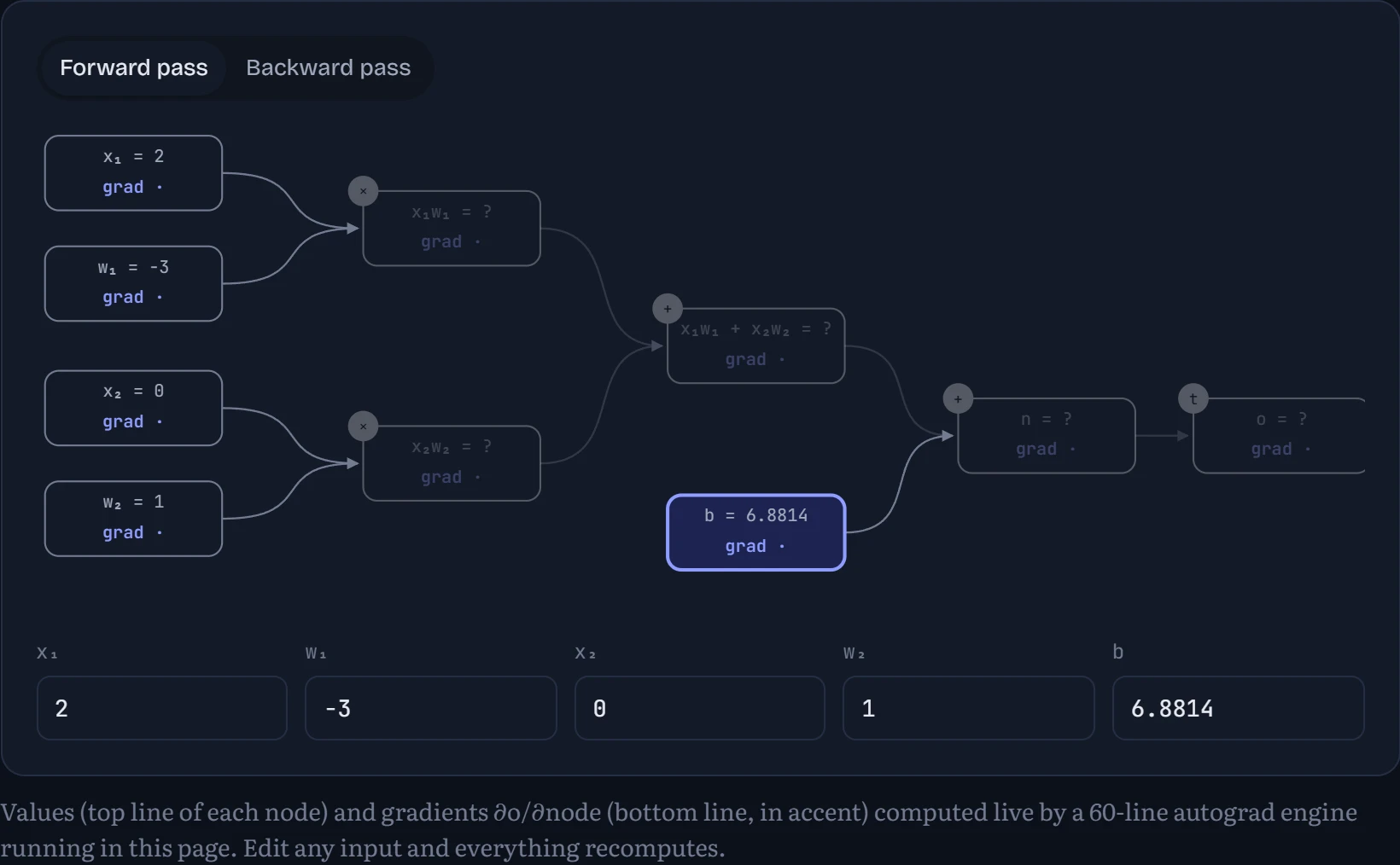
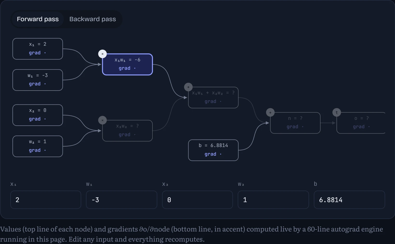
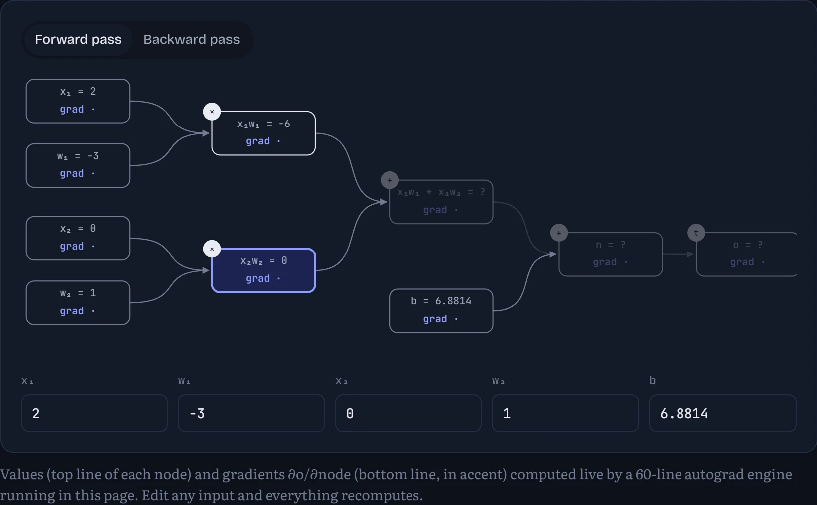
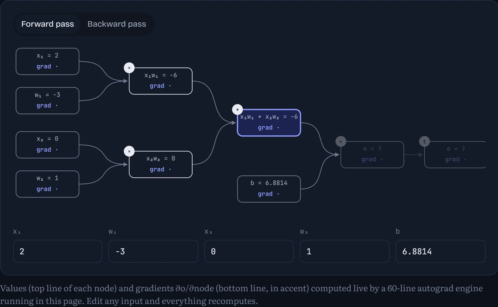
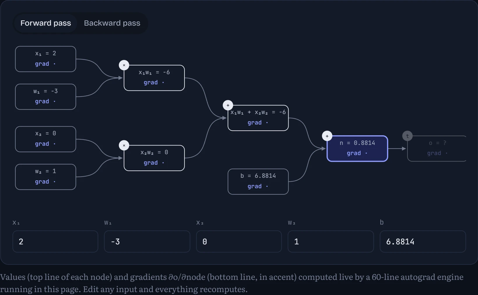
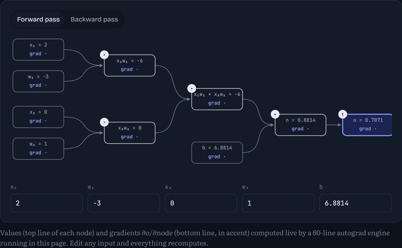
Notice that no node ever needed to know about the whole graph. Each one only knows its own local derivative: a “+” passes the gradient through unchanged, a “×” hands each input the other input's value times the incoming gradient, tanh multiplies by 1 − tanh². The chain rule says the gradient at any node is the product of local derivatives along the path back from the output. Backpropagation is just doing that product once per node, in the right order, reusing everything already computed. That's why computing all the gradients costs only a small constant times the forward pass, whether there are ten weights or ten billion.
Don't trust it. Check it.
You can always estimate a gradient the slow way: nudge one input by a tiny h, rerun the forward pass, and see how much the output moved. That's a finite difference. Here it is, live, against backprop:
| Input | Backprop ∂o/∂input | Finite difference (h = 10⁻⁶) | Difference |
|---|---|---|---|
x₁ | -1.49994397 | -1.49994397 | 9.7e-12 |
w₁ | 0.99996265 | 0.99996265 | 1.5e-10 |
x₂ | 0.49998132 | 0.49998132 | 7.7e-11 |
w₂ | 0.00000000 | 0.00000000 | 0.0e+0 |
b | 0.49998132 | 0.49998132 | 7.7e-11 |
They agree to about six or seven significant digits; the tiny leftover is the finite difference's own error, not backprop's. Finite differences need two forward passes per parameter, which for a 7-billion-parameter model is 14 billion forward passes for a single step. Backprop gives you all of them for roughly the price of two or three. That ratio is the entire reason deep learning is possible.
The engine: two rules and a sort
An autograd engine is surprisingly small. Every operation does two things when it runs forward: compute its output, and stash a little function that knows its local derivative. Then backward() needs just two rules.
Rule 1: visit nodes in reverse topological order. A node's gradient isn't final until every node that used it has passed gradient back. Sorting the graph so each node comes after its inputs, then walking it backwards, guarantees that.
Rule 2: accumulate with +=, never =. If a value is used twice, gradient arrives from both uses and must be summed. This is the multivariable chain rule, and getting it wrong is the classic first bug. See for yourself:
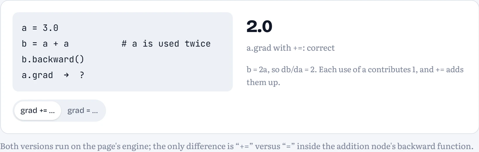
That's genuinely the whole engine. The Python version you'll write in Lab 5 is at the bottom of this page: about 60 lines, and it can train a neural network. PyTorch's autograd is the same idea, run over tensors instead of single numbers, with very fast kernels for each operation.
Batched: the same rules, as matrix shapes
A scalar engine is perfect for understanding and hopeless for speed. Real networks process a batch of B examples through each layer as one matrix multiplication. The rules stay identical; they just become shapes.
Nothing new happens here. A weight that connects input i to output j still gets the same “other input times incoming gradient” it got in the scalar graph; the matrix version just computes it for every weight and every example in one go, and adds up the contributions from all B examples. Writing it as matrix multiplications matters only because computers, and especially GPUs, are extremely fast at those. For a linear layer Y = X Wᵀ + b, with X of shape (B, in) and W of shape (out, in), the rules look like this:
forward     Y  = X · Wᵀ + b          (B, out)

backward    dW = dYᵀ · X             (out, in)     same shape as W, always
            db = dY summed over B    (out,)
            dX = dY · W              (B, in)       passed on to the previous layer

activation  dZ = dA ⊙ f′(Z)          tanh: f′ = 1 − tanh²   ReLU: f′ = 1 if Z > 0 else 0
loss        dLogits = (softmax − one_hot) / B    the p − y from the milestone
A handy sanity check: every gradient has exactly the shape of the thing it's the gradient of. If dW comes out (in, out), you transposed something. The playground at the top of the page uses exactly these five lines, in plain JavaScript, on all 300 points at once, every step.
Optimizers: what to do with a gradient
The gradient tells you which way is downhill right here. It doesn't tell you how far to go, and on real loss surfaces “downhill right here” is often a bad guide. The classic problem is a long, narrow valley: steep walls, gentle floor. Plain gradient descent bounces between the walls and crawls along the floor. Watch four optimizers race from the same starting point:
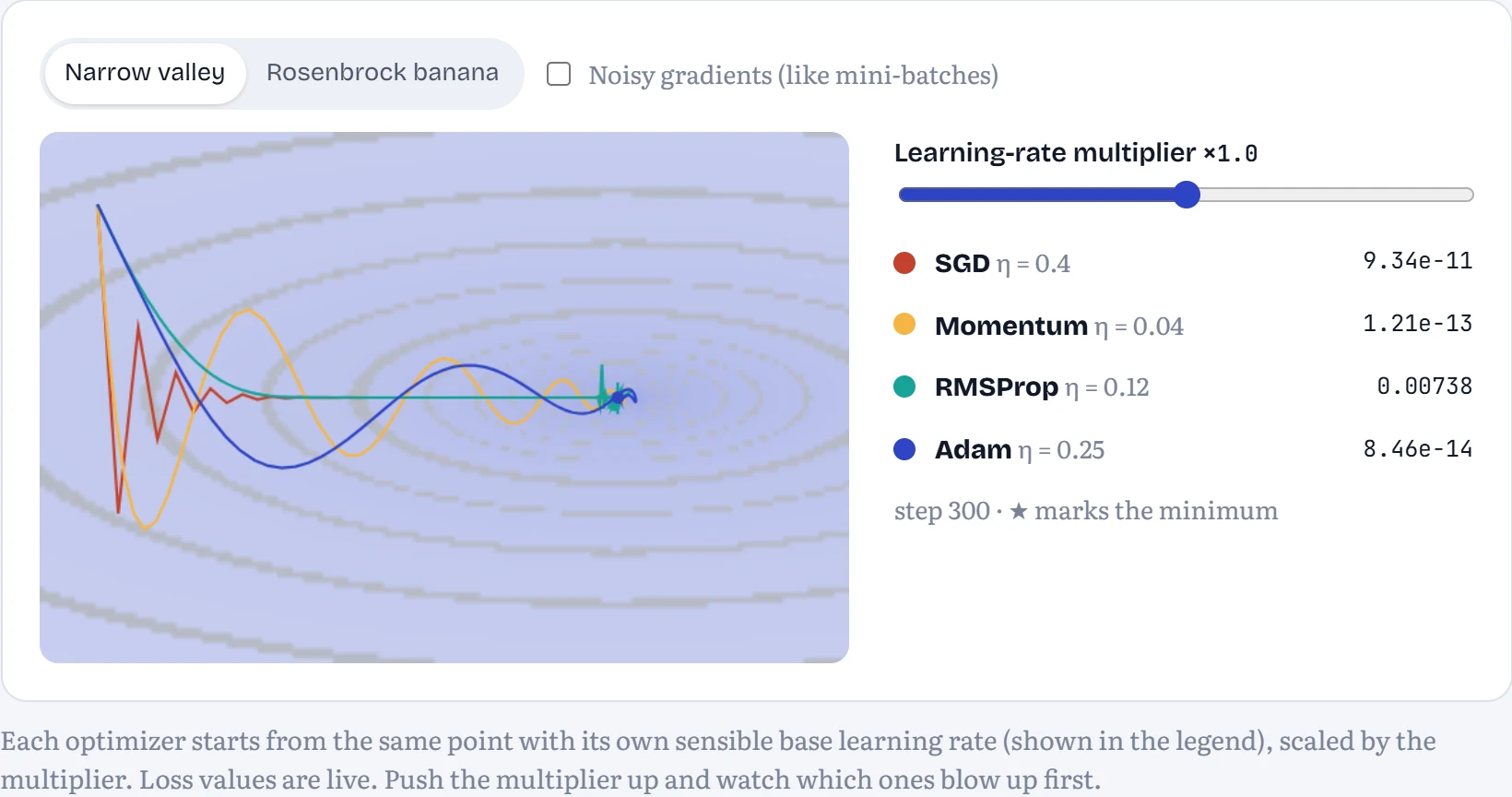
Imagine walking downhill in fog, only able to feel the slope under your feet. SGD takes a step straight down the local slope every time, which in a narrow valley means zigzagging from wall to wall. Momentum is a heavy ball instead of a walker: it keeps some of its previous speed, so the side-to-side pushes cancel out while the downhill push builds up. RMSProp gives every direction its own step size, taking small steps where the ground is steep and big steps where it's gentle. Adam does both at once. Here are the exact update rules behind each trail, where θ is a parameter, g its gradient and η the learning rate:
SGD        θ ← θ − η·g
Momentum   v ← β·v + g;          θ ← θ − η·v                          β = 0.9: a heavy ball that keeps rolling
RMSProp    s ← ρ·s + (1−ρ)·g²;    θ ← θ − η·g / (√s + ε)              each parameter gets its own step size
Adam       m ← β₁m + (1−β₁)g;  s ← β₂s + (1−β₂)g²;  bias-correct both;  θ ← θ − η·m̂ / (√ŝ + ε)
Momentum fixes the bouncing by averaging: the side-to-side components cancel out and the along-the-floor component adds up. RMSProp fixes the crawl differently, by dividing each parameter's step by how big its gradients usually are, so the steep direction gets small steps and the gentle one gets big steps. Adam does both, and corrects for the fact that its running averages start at zero. AdamW, which you used in the milestone, additionally applies weight decay directly to the weights instead of mixing it into the gradient, which interacts better with Adam's rescaling.
Adam is the default for training Transformers, and you'll use it almost everywhere. It isn't magic, though: on the Rosenbrock banana, watch how every method still has to creep along the curved valley floor.
Schedules: changing the step size during training
One learning rate for the whole run is rarely best. Early on, big steps make fast progress; near the end, big steps keep bouncing around the bottom of the valley. So training uses a schedule: step decay cuts the rate by 10× at fixed points, cosine glides it smoothly down to near zero, and warmup starts tiny and ramps up over the first few percent of training, which protects the network while its weights (and Adam's running averages) are still random. I trained the MNIST network for three epochs with SGD plus momentum under each schedule, at a sensible peak rate (0.1) and an aggressive one (0.4). How to read the chart: training loss over time; the small chart above each line shows the learning rate it was using.
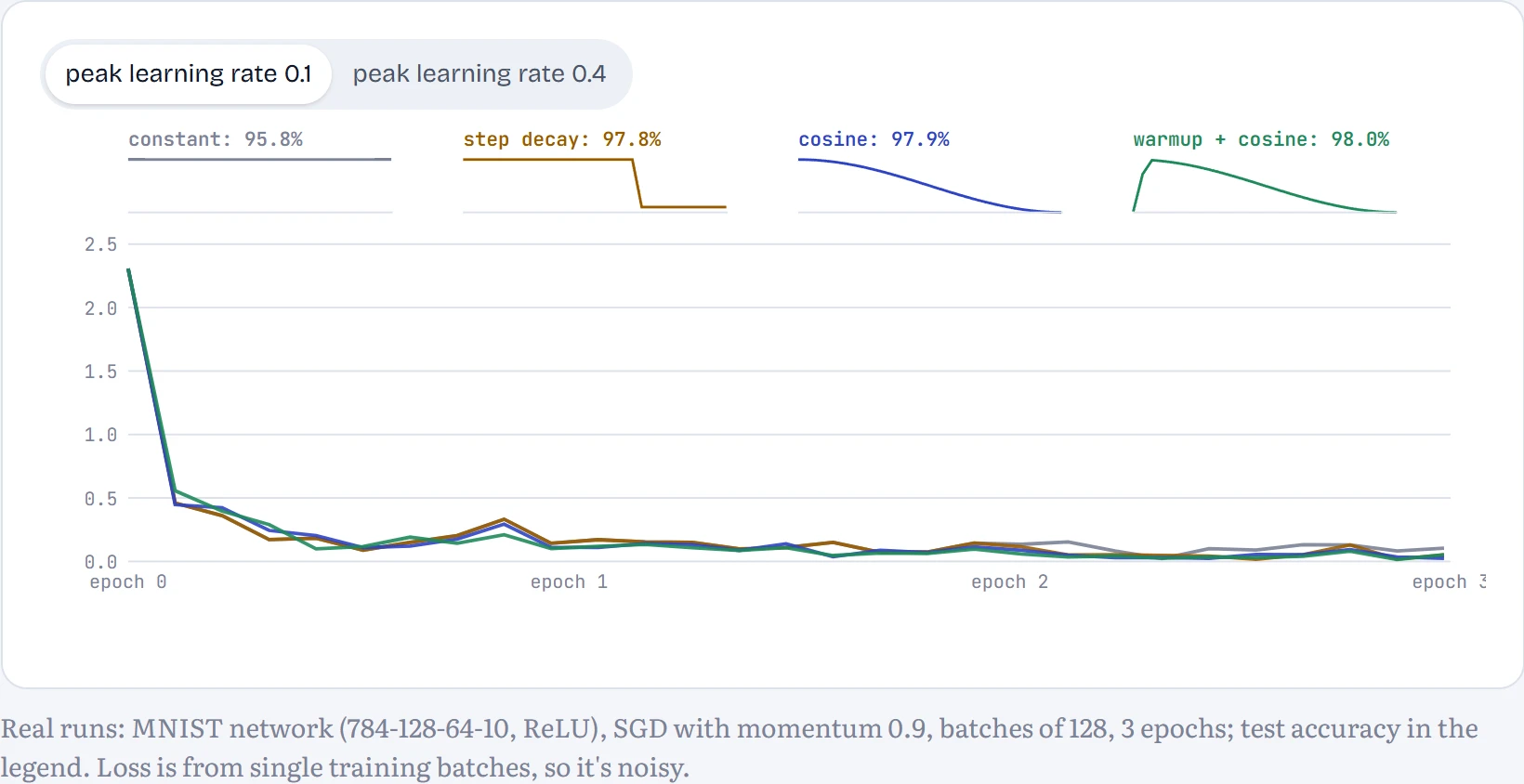
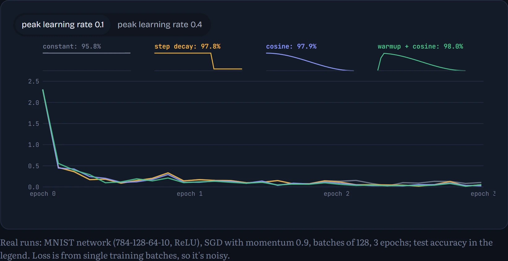
At the sensible rate (0.1), every schedule that decays beat the constant rate: constant 95.8%, step decay 97.8%, cosine 97.9%, warmup + cosine 98.0%. Shrinking the steps at the end lets the weights settle into the bottom of the valley instead of bouncing around it, worth about 2 points here. At the aggressive rate (0.4) every schedule failed, warmup included: all four ended at chance (11.3%). Warmup protects a network through its first, most fragile steps, which is where Transformers trained with Adam tend to blow up; it can't rescue a peak rate that is too high for the whole run. The peak rate matters most, which is why the milestone in Chapter 7 starts with a learning-rate sweep. Every large model trains with warmup followed by a decay, usually cosine (Chapter 10.6 adds the newer warmup-stable-decay schedule).
Batch size interacts with all of this. Bigger batches give a less noisy gradient per step, but for the same number of passes through the data they take fewer steps. How to read the table: the same network, two epochs with Adam at the same learning rate.
| Batch size | Update steps in 2 epochs | Seconds | Test accuracy |
|---|---|---|---|
| 16 | 7,500 | 24.2 | 97.0% |
| 128 | 938 | 2.8 | 96.2% |
| 1024 | 118 | 1.1 | 93.4% |
A batch of 1024 took only 118 steps and reached 93.4%; a batch of 128 took 938 steps and reached 96.2%; a batch of 16 took 7,500 steps and reached 97.0%, but at 8.7× the time of batch 128, because tiny batches can't keep the hardware busy. Large batches need a larger learning rate (and warmup) to make up for taking fewer steps; a common rule of thumb scales the rate with the square root of the batch size for Adam. Chapter 10 shows how big training runs pick their batch size.
Why deep networks refused to train
For years, networks deeper than a few layers mostly didn't train. Backprop was correct; the numbers just died on the way. Every layer multiplies the signal by its weights on the way forward, and multiplies the gradient by its weights (and its activation's slope) on the way back. Multiply by something a bit less than 1 twelve times and you have almost nothing. A bit more than 1, and you have an explosion.
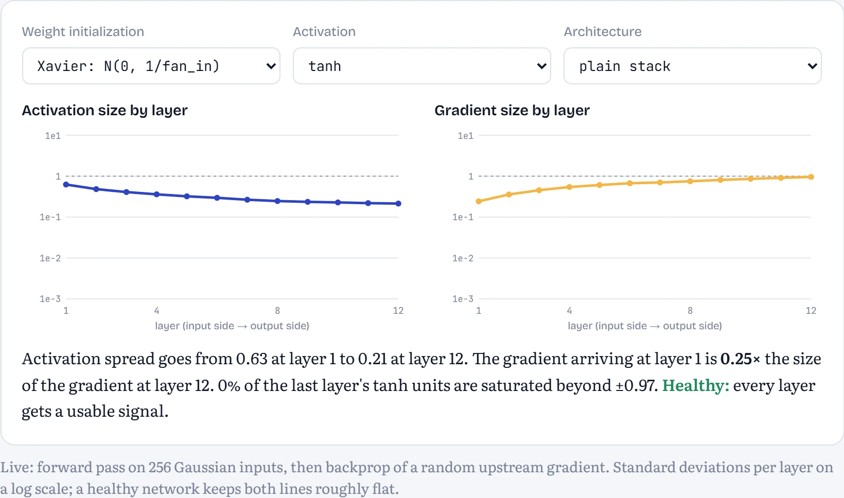
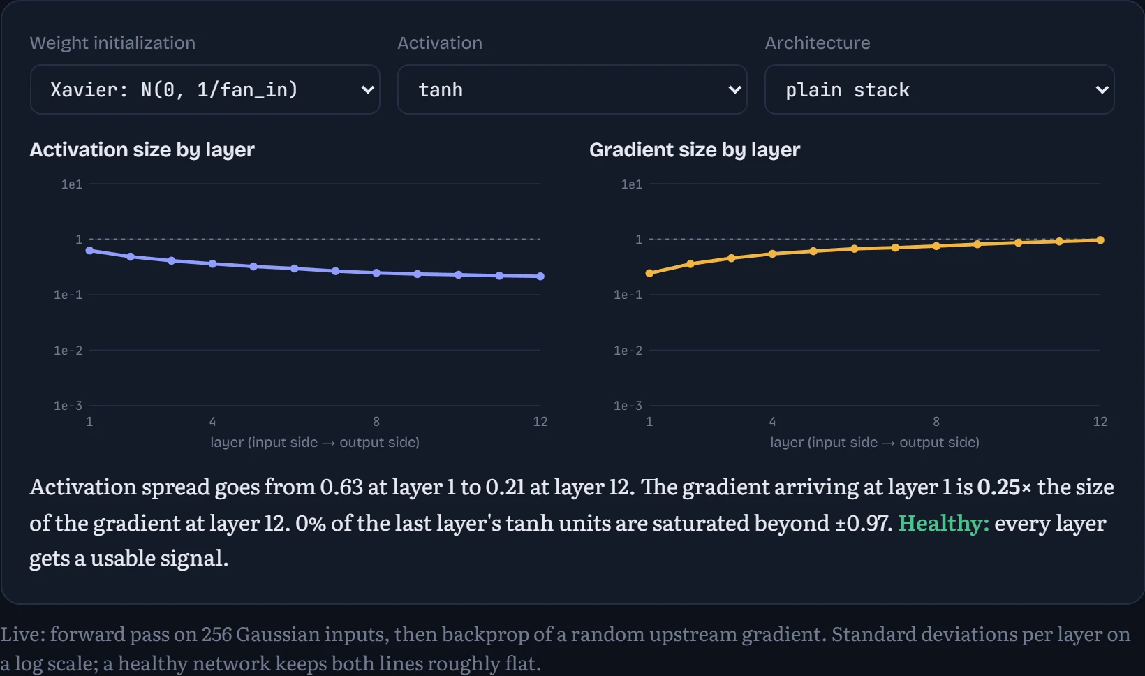
Here's a real 12-layer network, 128 units wide, on a batch of 256 random inputs. The page measures how big the activations and the gradients are at every layer.
How to read it: the left chart shows how big the numbers flowing forward are at each layer, from the input (left) to the output (right). The right chart shows how big the learning signal flowing backward is at each layer. The dashed line marks a size of 1. Flat lines near it are healthy. A line diving towards the bottom means the signal is vanishing; a line shooting up means it's exploding. The sentence under the charts reads the result out for you.
N(0, 1) with tanh. Most units pin to ±1, where tanh's slope is nearly zero. You might expect the gradient to vanish. It doesn't: it explodes going backwards, by a factor of thousands, because weights this large amplify whatever leaks through the few units that aren't saturated. I expected vanishing too when I first ran it. Either way, the network is untrainable.
N(0, 0.01²). The opposite failure. Every layer shrinks the signal, so by layer 12 the activations are around 10⁻¹², and the gradient reaching layer 1 is just as negligible.
Xavier with tanh. Weights scaled so each layer roughly preserves the size of its input. Both lines stay within a small factor across all 12 layers. Healthy.
Xavier with ReLU, then Kaiming with ReLU. ReLU throws away the negative half of its input, so with Xavier the signal halves in variance at every layer and fades. Kaiming doubles the weight variance to compensate (that's the 2 in 2/fan_in), and both lines go flat.
Then switch to residual. With h + f(h), the gradient always has a path that skips the layer, so it can't vanish however bad f is. It can still blow up if the weights are huge (try N(0, 1) again), and the activations grow with depth because every layer adds to them. Keeping that growth in check is LayerNorm's job, and it's the pre-norm design you'll meet in Chapter 9. Careful initialization, residual connections and normalization together are why 100-layer networks train today.
Continue the lesson
The whole lesson, with its drawings and its questions. 5 more sections after the ones above.