
mini_lm v1: a Bengio-style fixed-window character MLP, tanh-gain initialization and checkpointing
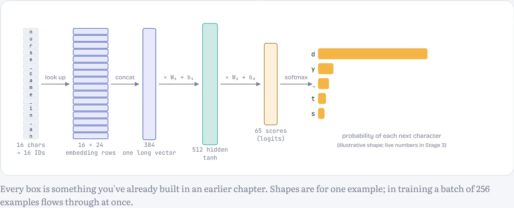
mini_lm v1 reads the last 16 characters, looks each one up in a table of learned vectors, joins them into one long vector, passes it through one hidden layer and scores every possible next character. It is the fixed-window design of Bengio and colleagues, trained, measured and saved properly.
What this page answers
How do you build a neural language model from scratch?
Slide a window over the text to get examples for free, embed each character, join the vectors, pass them through a hidden layer, score every next character, and train with cross-entropy loss. Read it in the lesson
Why does initialization matter for a neural network?
Weights drawn naively from a standard normal saturate the hidden layer before training starts. Scaling the hidden layer by the tanh gain over the square root of fan-in, and shrinking the output layer, spreads its outputs across the useful range. Read it in the lesson
The plan
Here's the whole machine before we build any of it. It reads the last 16 characters, looks each one up in a small table of learned vectors, glues those vectors into one long vector, pushes that through one hidden layer, and scores all 65 possible next characters. It's the design from Bengio and colleagues' 2003 paper that started neural language modelling, scaled to a laptop.
What you need
A laptop, Python, PyTorch, and about a megabyte of text. This page uses Tiny Shakespeare (1.1M characters of the plays), the same data the Chapter 9 lesson uses, so you'll be able to compare your v1 directly against a Transformer later. The full training run below took 64 s on a laptop CPU. No GPU required.
You'll write it in PyTorch, but you won't lean on anything you haven't built by hand. Autograd replaces the engine you wrote in Chapter 5, and you'll check it against your own derivation in Stage 3.
Data
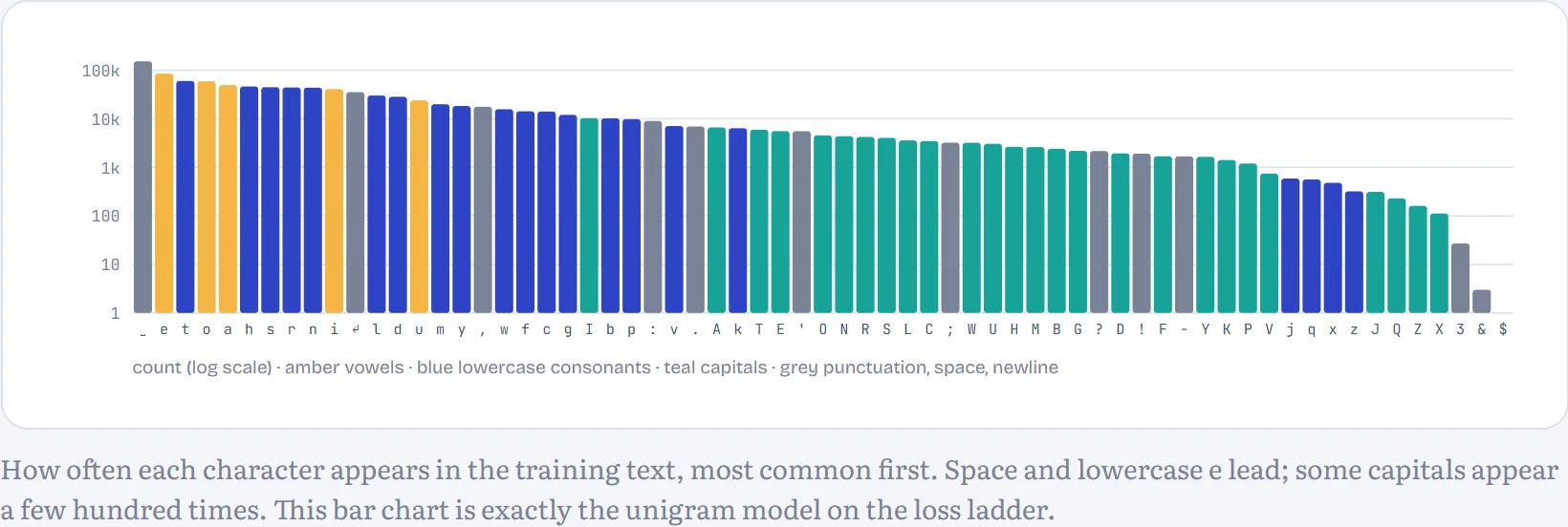
First, meet the data. The corpus has 1,115,394 characters drawn from an alphabet of just 65. That alphabet is the tokenizer: each character gets an ID from 0 to 64. You built a BPE tokenizer in Chapter 6, and it would work here too. Characters keep this first build small and let you see every prediction.
Slide a window, get examples for free
A language model needs (input, answer) pairs, and text hands them over for free. Take any 16 consecutive characters as the input; the 17th is the answer. Slide one step and you have another example.
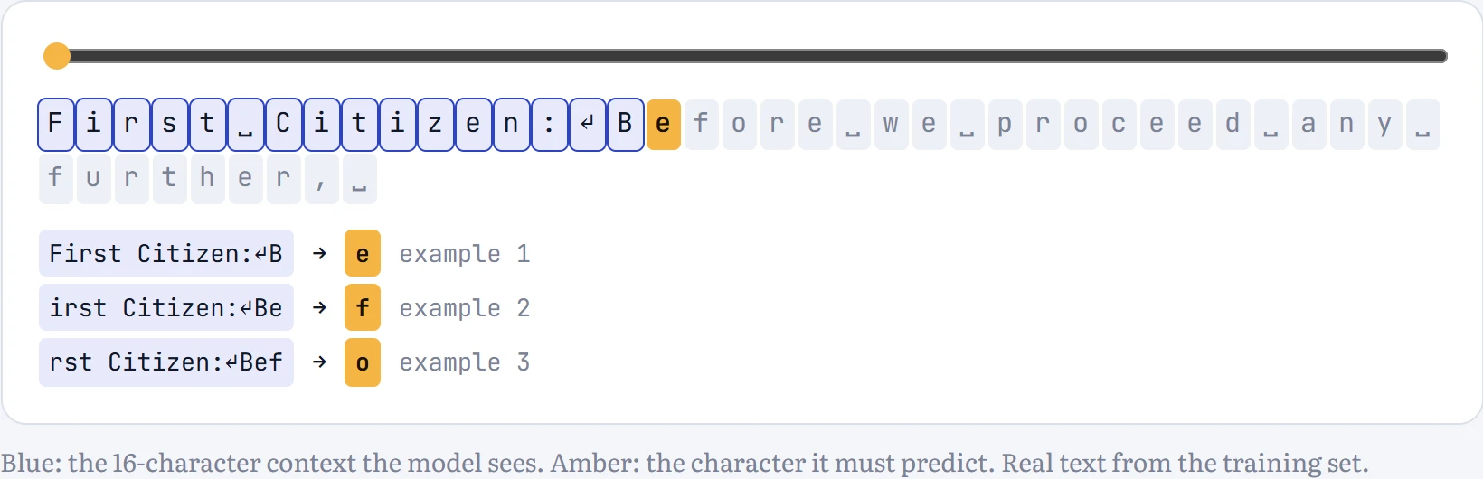
Predict first. The training split has about a million characters. With a 16-character window that slides one step at a time, roughly how many training examples is that?
- About 60,000 (one per window of 16)
- About 1,000,000
- About 16,000,000
Answer. About a million, one per position (exactly 1,003,838). The windows overlap, which is fine: each one asks a different question. We hold back the last 10% of the text as a validation set the model never trains on, and that split is by position, not random, so no window straddles the boundary and leaks answers.
✓
Checkpoint 1 You can print a batch: x has shape (256, 16), y has shape (256,), and decoding x[0] then y[0] gives 17 consecutive characters of real text.
The model
The model is three weight tensors and two bias vectors. Here's where every one of its parameters lives:
| Tensor | Shape | Parameters | Share |
|---|---|---|---|
| Embedding table | 65 × 24 | 1,560 | 0.7% |
| Hidden layer W₁ + b₁ | 384 × 512 + 512 | 197,120 | 85.0% |
| Output layer W₂ + b₂ | 512 × 65 + 65 | 33,345 | 14.4% |
| Total | 232,025 | 100% |
Notice where the bulk is: the first layer, because it reads all 16 × 24 = 384 numbers of the window. Double the context and that layer doubles. Hold that thought for Stage 6.
The embedding table deserves a second look. Looking up row 17 is exactly what multiplying a one-hot vector by the matrix does (Chapter 2.3), just without wasting 64 multiplications by zero. And because the table is trained, characters that behave alike end up with similar rows. You'll see that happen in Stage 4.
Initialization: the bug that doesn't crash
Before training a single step, there's a check that catches a surprising number of bugs.
Predict first. A freshly initialized model should know nothing, so it should spread its bets evenly over all 65 characters. What loss should step 0 show?
- 0
- 1
- ln(65) ≈ 4.17
- 65
Answer. ln(65) ≈ 4.17: probability 1/65 on the right answer, and −ln(1/65) = ln 65. Now look at what two different initializations actually gave.
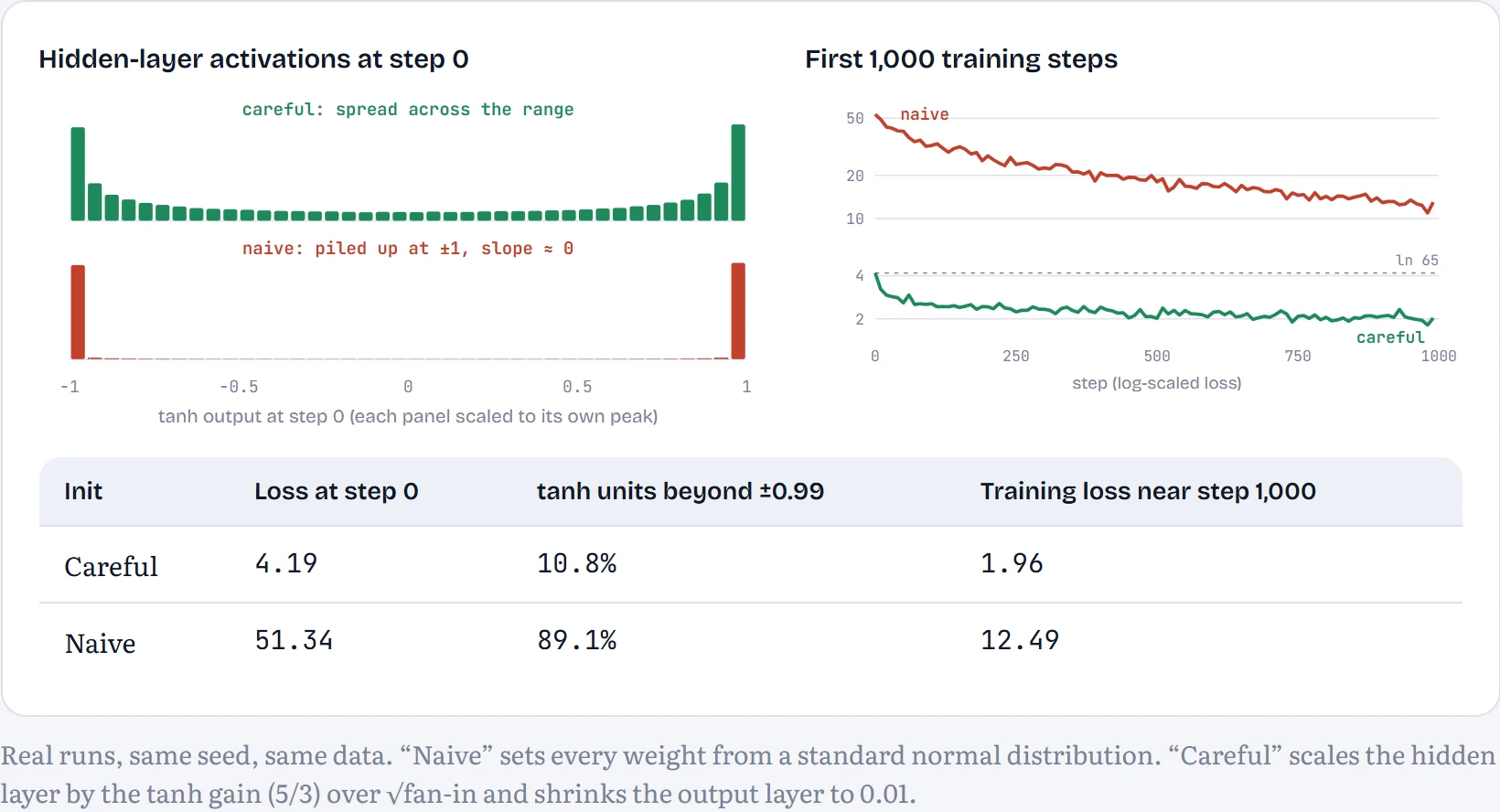
How to read it: the left panel shows the hidden layer's outputs before any training. The careful version (green) spreads them across the whole range; the naive one (red) piles almost all of them up at −1 and +1, the flat ends of tanh where learning stalls. The right panel is the training loss for the first 1,000 steps. The naive run starts enormously high and spends its first stretch just undoing its own bad start. The table puts numbers on both.
A badly initialized model is like a student who walks into the exam already certain of a lot of wrong answers. Before they can learn anything, they have to unlearn that confidence, and that wastes time. A well-initialized model starts out humble, spreading its guesses evenly, so every bit of training goes into learning.
The naive model starts out confidently wrong. Its huge random output weights make it put most of its probability on a few arbitrary characters, so the first loss is far above 4.17. Worse, most of its tanh units are pinned at ±1, where the slope of tanh is nearly zero, so gradients barely flow. It spends its first few hundred steps just undoing its own overconfidence: the famous “hockey stick” loss curve. That's wasted compute, and in deeper networks it can stop training altogether.
✓
Checkpoint 2 Your step-0 loss is within about 0.1 of ln(vocab size), and only a small minority of tanh activations sit beyond ±0.99 (ours: 11%, versus 89% with naive init).
The training loop
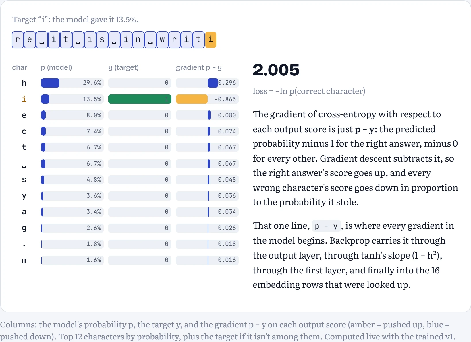
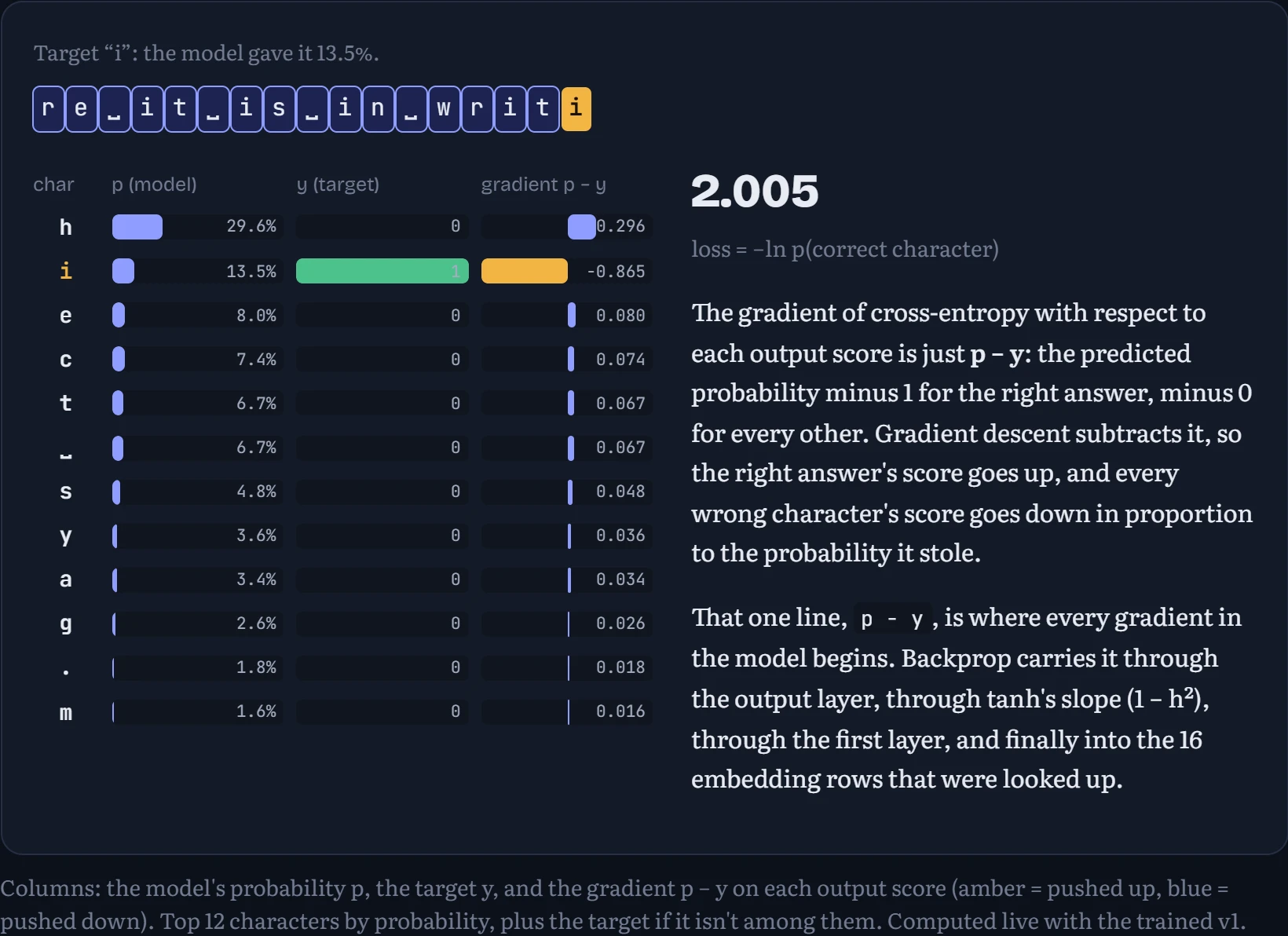
One training step, for real. Below, one example from the text: what the model predicts, what the loss is, and the exact gradient that comes back into its output scores.
The loss is a measure of surprise: −ln of the probability the model gave to the character that actually came next. Give the right answer 50% and the loss is 0.69. Give it 10% and it's 2.3. Give it 1% and it's 4.6. A model that's confidently wrong gets punished hard, and one that's confidently right barely at all. Training is just nudging every weight, a little at a time, in the direction that would have made the right answer less surprising.
Trust, but verify: check autograd against your own math
The milestone asks you to derive one layer's gradients by hand and compare them with PyTorch. I derived every layer, including the scatter-add back into the embedding table, and compared on a real batch in 64-bit floats:
| Gradient | Largest value | Largest difference, mine vs autograd |
|---|---|---|
fc2.weight | 1.44e-1 | 2.1e-17 |
fc2.bias | 1.89e-1 | 6.9e-18 |
fc1.weight | 7.50e-3 | 1.7e-18 |
fc1.bias | 3.60e-3 | 8.7e-19 |
emb.weight | 5.73e-3 | 3.5e-18 |
Differences around 10−17 mean the two agree to the last bit of floating-point precision. If yours are around 10−2, you have a real bug, usually a missing 1/B from averaging over the batch or a transposed matrix.
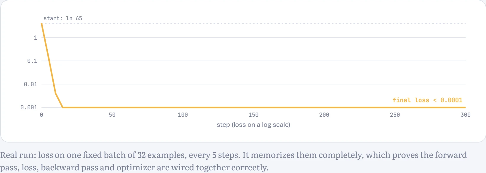
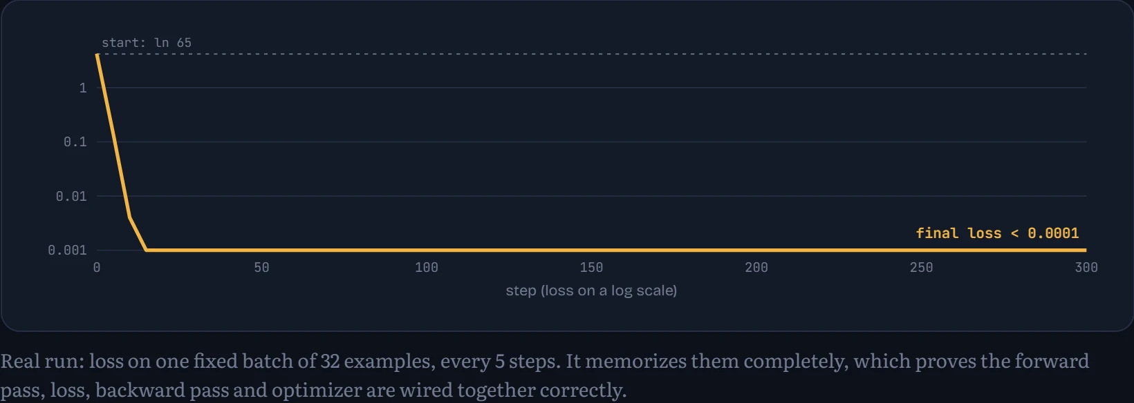
The single most useful test: can it memorize 32 examples?
Before spending minutes on a full run, train on one fixed batch of 32 examples and nothing else. A correct model and loop should drive that loss to almost zero. If it can't, there's no point training on a million examples: something is broken.
The learning-rate schedule, and clipping
Two lines in the training loop deserve a closer look. The schedule lowers the learning rate along a cosine curve to a tenth of its starting value, and clip_grad_norm_ caps the size of each update. Are they pulling their weight? I re-ran the milestone model with a constant rate, with cosine decay, and with a short warmup before the cosine, at the normal rate (0.003) and at rates 3× and 10× higher, plus one run with clipping switched off. How to read the chart: validation loss during training (lower is better).
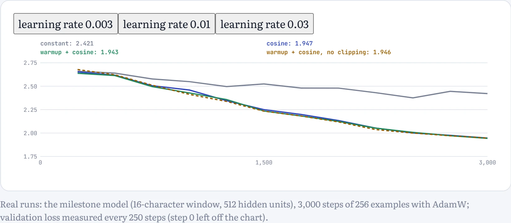
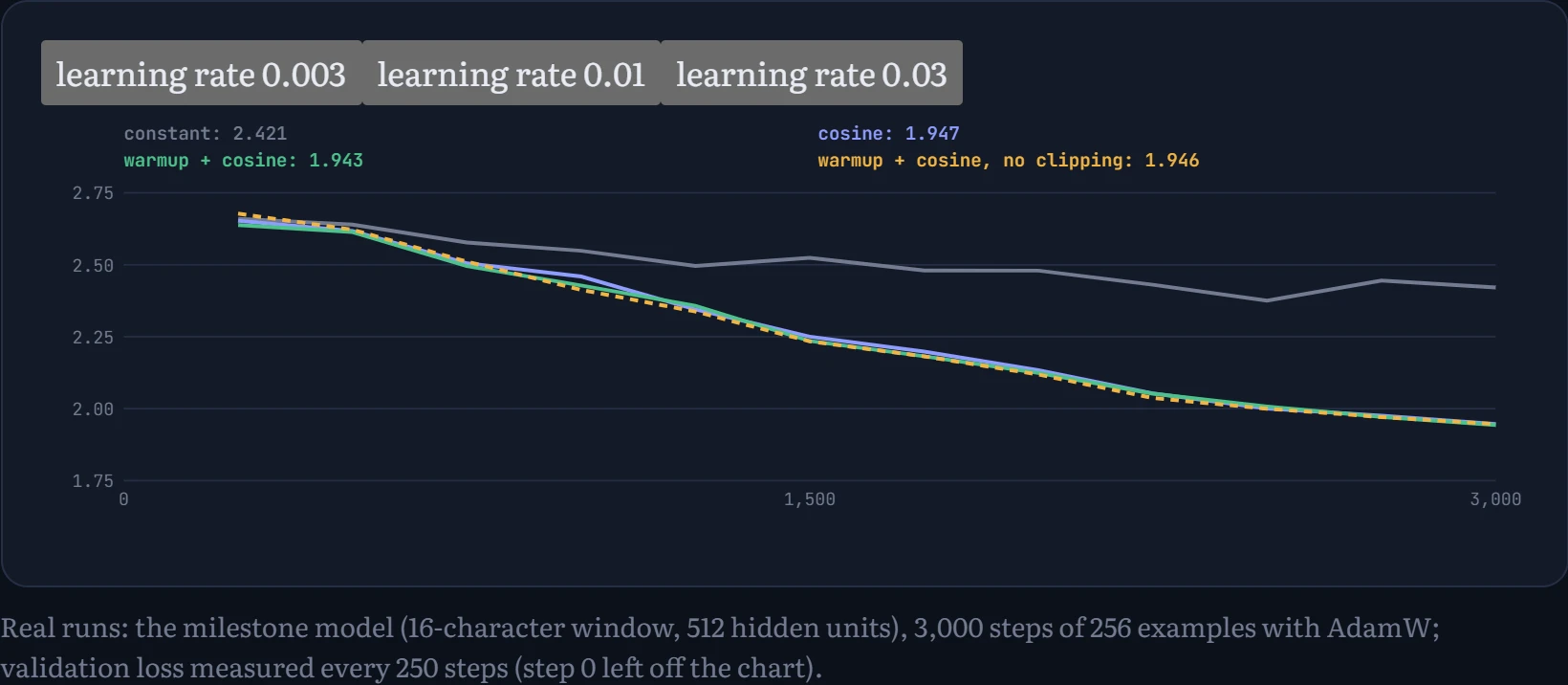
At the normal rate, cosine decay ended at 1.872 against 1.991 for a constant rate: shrinking the steps at the end is worth about 0.17 bits per character for free. The higher the rate, the more it matters. At 0.01, constant ended at 2.421 and cosine at 1.947; at 0.03, 4.092 against 2.313. Warmup and clipping barely changed anything here (2.288 with warmup, 2.307 without clipping): this small MLP with careful initialization has no fragile start and no exploding gradients. They're insurance, cheap to keep, and they become essential in the deeper Transformers of Chapter 9, where a single bad batch early on can wreck a run.
✓
Checkpoint 3 Hand-derived and autograd gradients match to at least 6 significant digits, and one batch of 32 examples overfits to a loss under 0.05.
Watching it learn
Now the real run: 8,000 steps, batches of 256, AdamW at a peak learning rate of 0.003 with cosine decay, gradient clipping at 1.0, 64 s on 6 CPU threads. Each checkpoint shows what the model wrote at that moment.
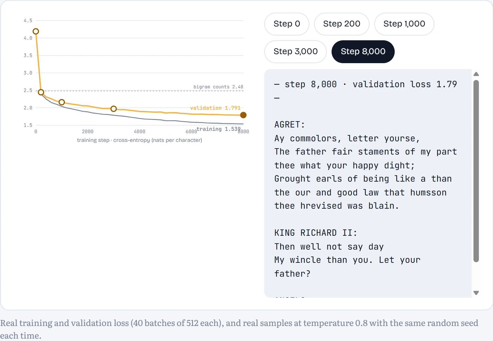
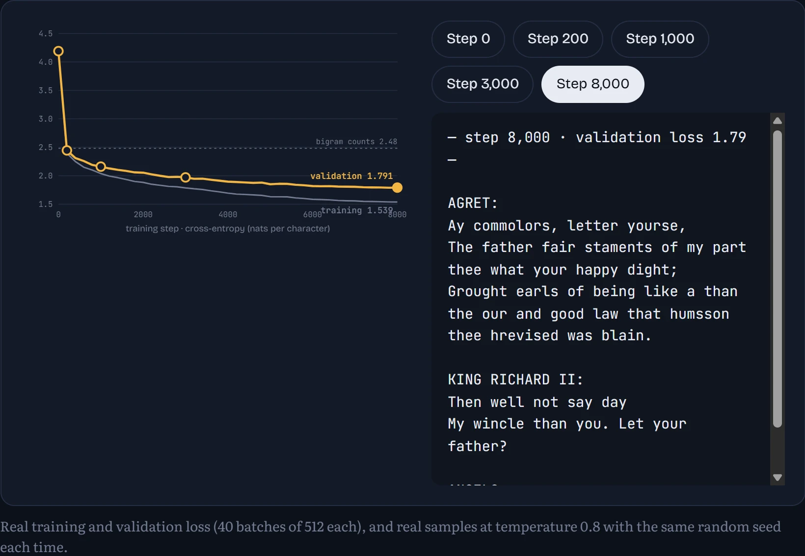
Read the samples in order and you can watch the model pick up the structure of the text, from the bottom up. First the character frequencies. Then spaces at roughly word-length intervals. Then real short words, then the NAME: line that starts every speech, then plausible words and punctuation. What it never gets is a sentence that means something. With 16 characters of memory, it never could.
What did the embedding table learn?
Each character's learned vector has 24 numbers. Squash them down to 2 (with PCA, Chapter 2.5) and plot. Its five nearest neighbours in the full 24-dimensional space tell more than the flat picture can.
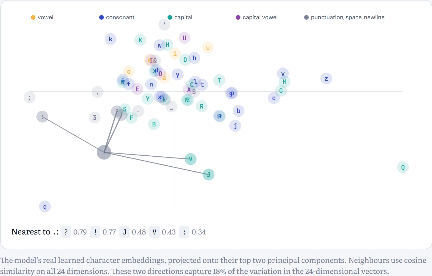
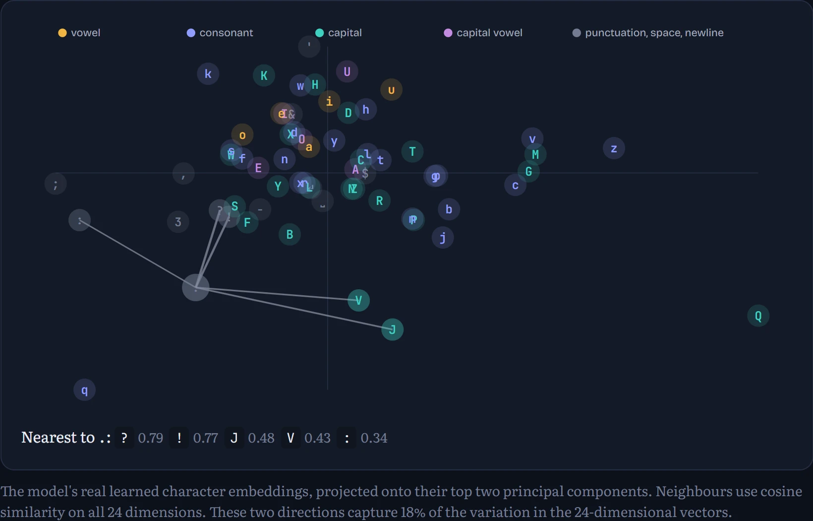
The broad strokes are visible even in 2-D. Lowercase letters crowd together, capitals spread out to one side, and punctuation and whitespace sit apart. But the projection keeps only a small share of the variation (see the caption), so most of the structure lives in the other 22 dimensions. The neighbour lists are more honest than the picture: characters are grouped by how they behave in text, which is all the model ever had to go on.
Three experiments worth running yourself
Each experiment below changes one thing and keeps everything else fixed. Make your guess before you look.
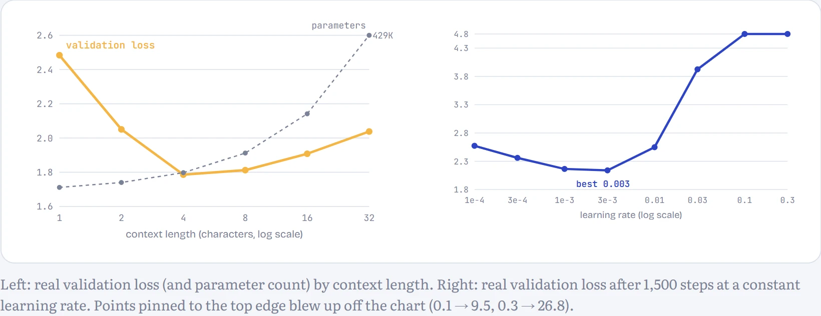
Predict first. We trained the same model with windows of 1, 2, 4, 8, 16 and 32 characters (3,000 steps each). Does more context always help?
- Yes, steadily
- It helps, then levels off
- It helps, then makes things worse
Answer. It helps, then makes things worse. I expected “levels off” myself, so this one surprised me too. One character of context gives 2.48, basically a bigram with a hidden layer. The best window is 4 characters at 1.79. Past that, validation loss climbs: 1.91 at 16 and 2.04 at 32.
It isn't overfitting, because training loss gets worse too (1.60 at 4 versus 1.83 at 32). Every new slot brings its own block of first-layer weights that has to be learned from scratch (the dashed line), while characters far back carry little useful signal. With a fixed budget of 3,000 steps, the bigger model just learns more slowly. Our main model uses 16 characters and trains for 8,000 steps, which recovers most of the gap (1.79). And to be honest about it: I picked 16 before running this sweep. The cheap experiment should come before the expensive run.
How to read the two charts: on both, lower is better. On the left, each dot is a model trained with a different window length; the amber line is its validation loss, and the dashed grey line is how many parameters it needed. On the right, each dot is the same model trained with a different learning rate, on a log scale from very cautious (left) to very aggressive (right).
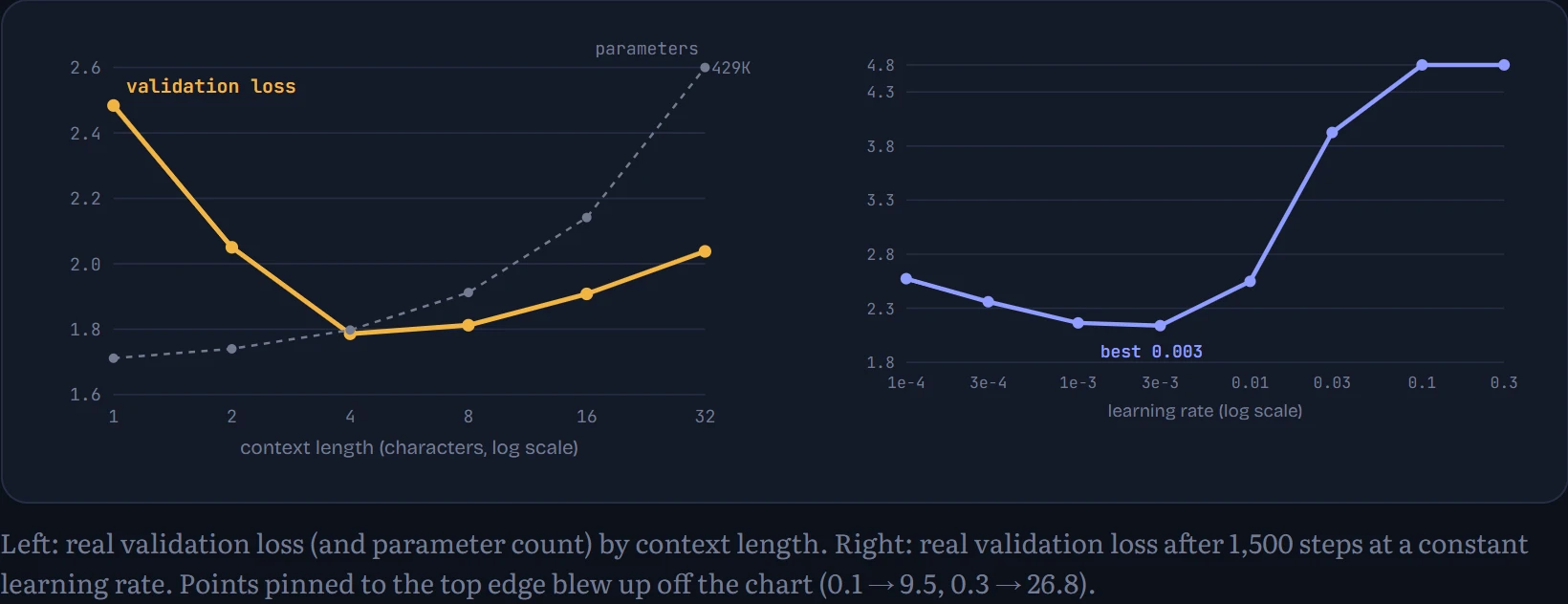
Learning rate has the classic U shape. Too low and the model barely moves in 1,500 steps. Too high and Adam's updates overshoot, the loss bounces around, and at the extreme it explodes. The sweet spot here is around 0.003 (validation 2.09 after 1,500 steps). Every new model and dataset needs this sweep. It takes minutes and saves hours.
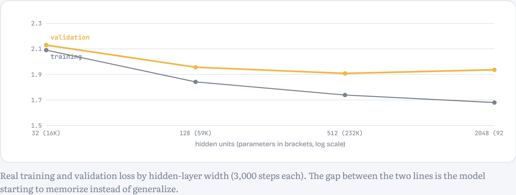
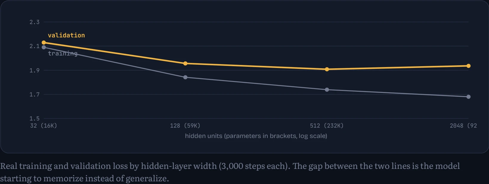
Width buys capacity. Going from 32 to 512 hidden units takes validation loss from 2.13 to 1.91. At 2048 units it gets worse on validation (1.94) even though training loss keeps falling (1.68): textbook overfitting. More capacity only helps if you have the data to fill it, which is a theme that comes back hard in Chapter 10's scaling laws.
✓
Checkpoint 4 Validation loss beats the count-based bigram from Chapter 1 by a clear margin, and you've run at least one sweep of your own and written down what you expected first.
Continue the lesson
The whole lesson, with its drawings and its questions. 6 more sections after the ones above.