
Multimodal models: ViT patches, CLIP contrastive learning, CTC speech recognition and DDPM diffusion
A transformer does not know what text is: it takes a list of vectors and gives back a list of vectors. Cut an image into square patches or sound into 25-millisecond slices, turn each piece into a vector, and the same machine sees and hears. Diffusion models then learn to generate images by removing noise.
What this page answers
How does a vision transformer read an image?
It cuts the image into a grid of square patches, flattens each patch's pixels into a list of numbers and multiplies by a learned matrix, so each patch becomes one vector, like a token. Read it in “Seeing: an image is sixteen words”
What is CLIP?
A model trained so that pictures and their captions land close together in one shared vector space, which lets it match images and text. Read it in “CLIP: one space for pictures and words”
Everything becomes a sequence of vectors
Here's the idea that makes this whole chapter possible. A Transformer doesn't know what text is. It takes in a list of vectors, lets every vector look at every other one, and gives back a list of vectors. In Chapter 6 we turned text into that kind of list by chopping it into tokens and looking each one up in an embedding table. If you can chop anything into pieces and turn each piece into a vector, the same machine works on it.
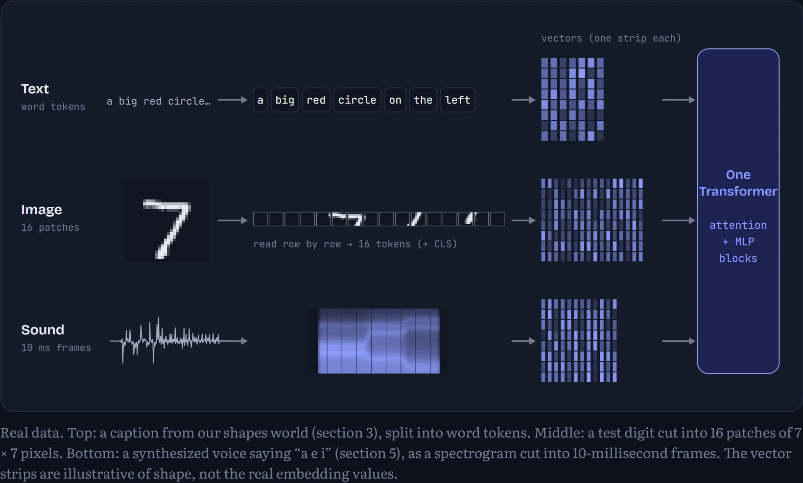
For a picture, the pieces are small square patches: cut the image into a grid, flatten each square's pixels into one long list of numbers, and multiply by a learned matrix to get a vector. For sound, the pieces are short slices of time: measure how much of each pitch is present in every 25-millisecond window, and each window becomes a vector. The figure below does exactly that to three real inputs from this lesson. How to read it: each row is one kind of input. Follow it left to right: the raw input, the pieces it's cut into, and then a column of vectors (drawn as little strips of colour, one cell per number) that all go into the same kind of model.
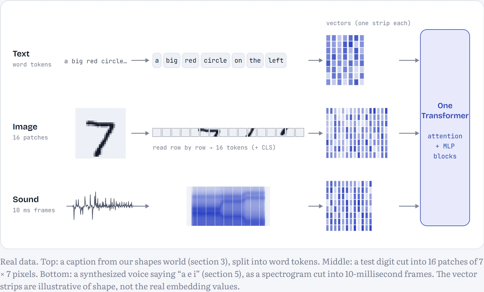
Once everything is a list of vectors, mixing senses is almost easy: put image vectors and word vectors in the same list, and attention can connect “the red one” to the red pixels. That's the whole trick behind models that can look at a photo and talk about it. The hard part, and most of this chapter, is getting the vectors to mean compatible things, and teaching models not just to understand images and sound but to make them.
Seeing: an image is sixteen words
Let's build the simplest possible seeing Transformer and find out what it learns. Our images are the handwritten digits from Chapter 5 (MNIST), 28 × 28 pixels. The recipe, called a Vision Transformer or ViT, has four steps:
1. Cut the image into a 4 × 4 grid of patches, each 7 × 7 pixels, so 49 numbers per patch. 2. Embed each patch by multiplying its 49 numbers by a learned matrix, giving 64 numbers: this is the patch's “word vector”. 3. Add position: each of the 16 slots gets its own learned vector added on, because attention by itself has no idea which patch was where (Chapter 8). 4. Add one extra token at the front, called CLS (for “classify”), that isn't any patch at all. It's an empty notepad. After four Transformer blocks, during which it can attend to all the patches, we read the answer off it.
Ours has 139,018 parameters: 64-number vectors, 4 attention heads, 4 blocks. I trained it for 8 passes over the 60,000 training digits, with small random rotations, zooms and shifts mixed in so it can cope with your handwriting. That took 11 minutes on a laptop CPU, and it scores 98.8% on the 10,000 test digits it never saw.
In the lesson's live demo, a drawing is shrunk and centred the way MNIST digits are and cut into the 16 patches the model reads. Bars show the model's confidence in each digit.
The demo's attention shading is telling: it usually lights up the patches where the strokes that distinguish this digit sit, like the closed loop of a 9 versus the open top of a 4, and largely ignores the empty corners. Nobody told it to. The only training signal was “this image is a 9”, and paying attention to the informative patches is simply what made that prediction work. (Attention maps are a hint about what the model used, not a full explanation; we'll come back to that in Chapter 15.)
Predict first. Take every test image, cut it into its 16 patches, and shuffle them into a random order, the same shuffle for every image. The patches keep their contents; only their arrangement is scrambled. What happens to the ViT's accuracy?
- Barely changes: attention doesn't care about order
- Drops a little
- Collapses
Answer. It collapses. With the patches scrambled, accuracy fell from 98.8% to 30.2%. If you picked “barely changes”, you had the right instinct about attention itself: on its own it really is blind to order. To prove it, I trained an identical twin with no position embeddings. Shuffling made no difference to it at all (96.0% shuffled, 96.0% unshuffled), because without positions every patch is just an item in a bag. So the collapse of the first model tells you it was relying heavily on where each patch sits.
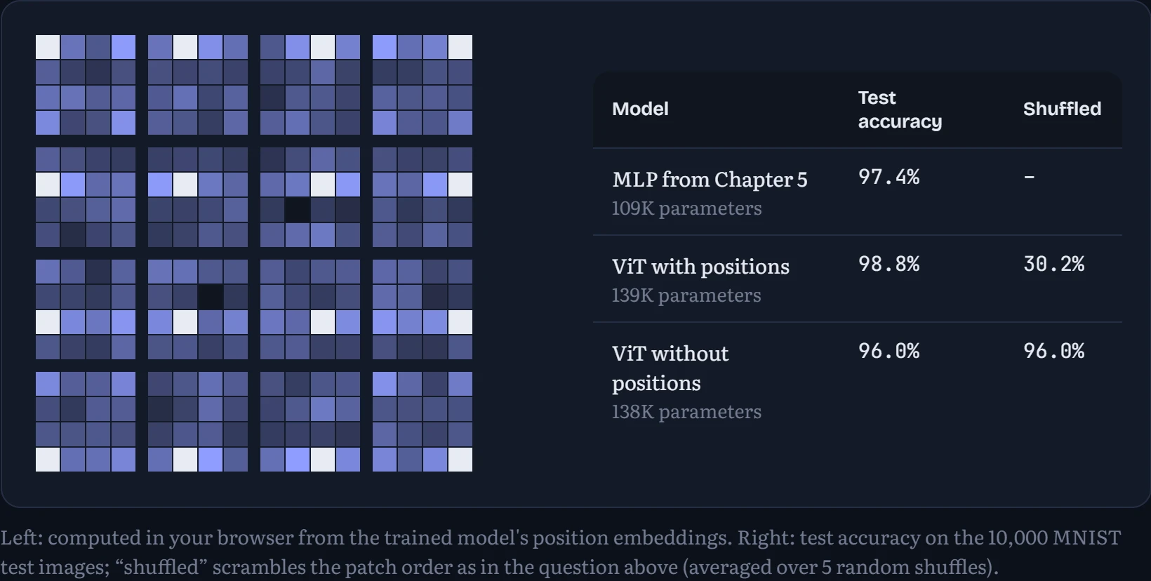
So where does the model keep its knowledge of the layout? In those 16 learned position vectors. We never told it the patches form a 4 × 4 grid; it just got one arbitrary vector per slot to tune during training. Below, I've compared every slot's position vector with every other slot's. How to read it: the big grid has one small map per patch slot, laid out where that patch sits in the image. Inside each small map, the solid cell is that slot itself, and every other cell is brighter the more its position vector points in the same direction as that slot's (cosine similarity, shaded from the least similar pair in the model to the most similar).
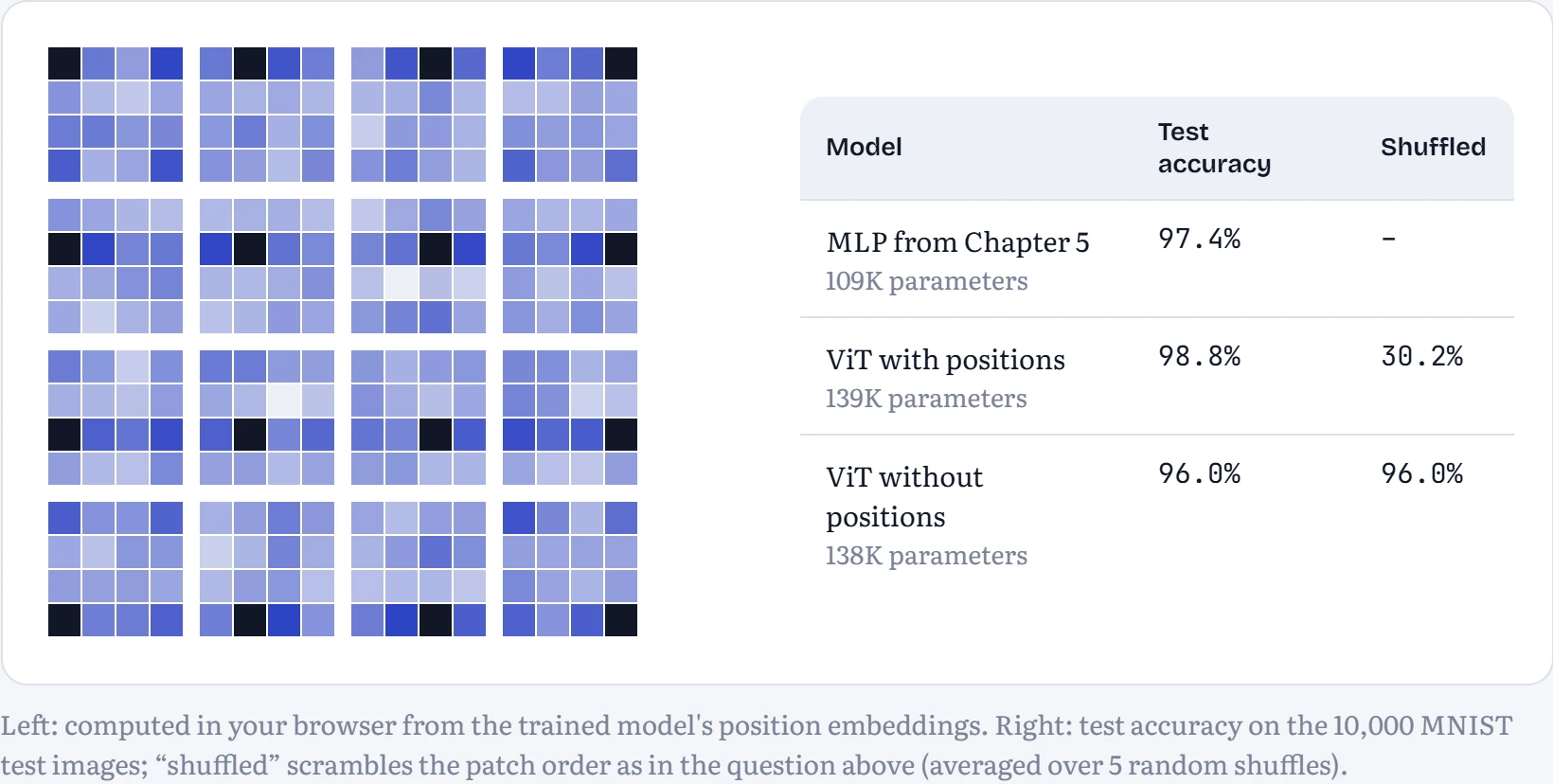
I expected a tidy picture here, and didn't get one. In the original ViT paper, big models trained on millions of photos learn position vectors where neighbouring patches look alike, so each small map lights up in a neat blob around its own slot. Ours learned something cruder. The clearest pattern is rows: slots in the same row have fairly similar position vectors (average similarity 0.30), while slots in the same column (-0.07) or in a different row and column (-0.15) don't. Look along each small map's row of cells and you'll see it. So this model mostly encodes “which row am I in” as a shared direction, and tells slots within a row apart in other, less visible ways: no two slots share a vector (the most similar pair reaches only 0.61), and the shuffle test proves the model uses them. A 4 × 4 grid of digit patches is a tiny world, and the model found a layout code that's good enough for it, not the textbook one.
The table puts the ViT in context. It beats the plain MLP from Chapter 5 (98.8% against 97.4%) with more parameters, partly thanks to the training augmentation the MLP didn't get. The position-free twin reaches 96.0% with no idea where anything is, which tells you how much a digit's identity is written in its patches' contents alone: a patch containing a tight curve or a sharp corner already narrows things down a lot.
How real vision models learn
A ViT has fewer built-in assumptions about images than the convolutional networks (CNNs) that ruled vision for a decade. A CNN slides the same small filter across the whole image, so it assumes from the start that nearby pixels matter together and that a cat is a cat wherever it appears. A ViT has to learn those facts, as ours did with its position map. The price is data: the original ViT paper (Dosovitskiy and colleagues, 2020) found ViTs lost to CNNs when trained on about a million images and won only at around 300 million. The payoff is that the same architecture scales like language models do.
Labelled images are expensive, so modern vision models mostly learn from unlabelled ones, in two main ways. Contrastive methods show the model two altered views of the same photo (cropped, recoloured) and train it to give them similar vectors while keeping other photos apart; DINO and SimCLR work this way, and you'll meet a cousin, CLIP, in the next section. Masked methods hide most of the patches, as much as 75% in the MAE paper (He and colleagues, 2021), and train the model to fill in the missing pixels, exactly like a language model filling in missing words. Either way, the model ends up with general-purpose image features that are then fine-tuned for specific jobs: detection (draw a box around every object and name it, as in DETR, which treats the list of boxes as a set of output tokens) and segmentation (label every pixel, as in Meta's Segment Anything).
CLIP: one space for pictures and words
A ViT can learn to say “this is a 9”, but only for the ten labels it was trained on. What if you want a model that understands any description: “a small dog on a red sofa”? You can't make a label for every possible sentence. The trick, from OpenAI's CLIP (Radford and colleagues, 2021), is to stop predicting labels altogether and instead train two encoders, one for images and one for text, so that a picture and its caption land at the same point in a shared space of vectors.
To see it clearly, I built a tiny world where I know the right answer to everything: 32 × 32 pictures of coloured shapes, each with a caption generated from what's in it. There are 5 colours, 4 shapes, 2 sizes and 4 positions, and some pictures have two objects side by side. Here are some real training examples:
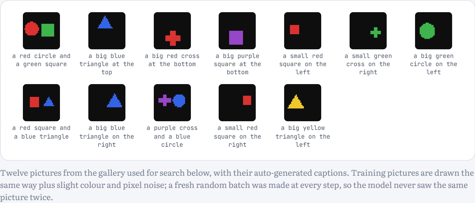
Training works like this. Take a batch of 128 pictures and their 128 captions. Encode all of them, scale every vector to length 1, and compare every picture with every caption (the dot product, which for unit vectors is the cosine similarity from Chapter 6). That gives a 128 × 128 grid of scores. The correct pairs sit on the diagonal. The loss is plain cross-entropy, applied twice: each row should pick out its own caption from the 128 candidates, and each column should pick out its own picture. Every wrong pairing in the batch acts as a free counter-example. A learned temperature multiplies the scores before the softmax, controlling how sharply the model commits.
Here's that grid for eight pictures, before and after training. How to read it: rows are pictures, columns are captions, in matching order, so the correct pairs are the diagonal. Darker blue means a higher similarity score. Before training, every score is about the same, a featureless mush. After training, the diagonal should stand out.
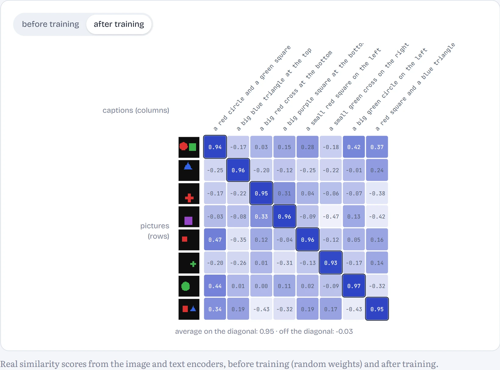
Because both encoders put their outputs in one space, you can search pictures with any sentence: encode the text, and rank pictures by how close they are. Below, the real text encoder ranks a gallery of pictures it was never trained on. How to read it: the pictures are sorted best match first, and the number under each is its cosine similarity to your query (1 would be identical direction, 0 unrelated).
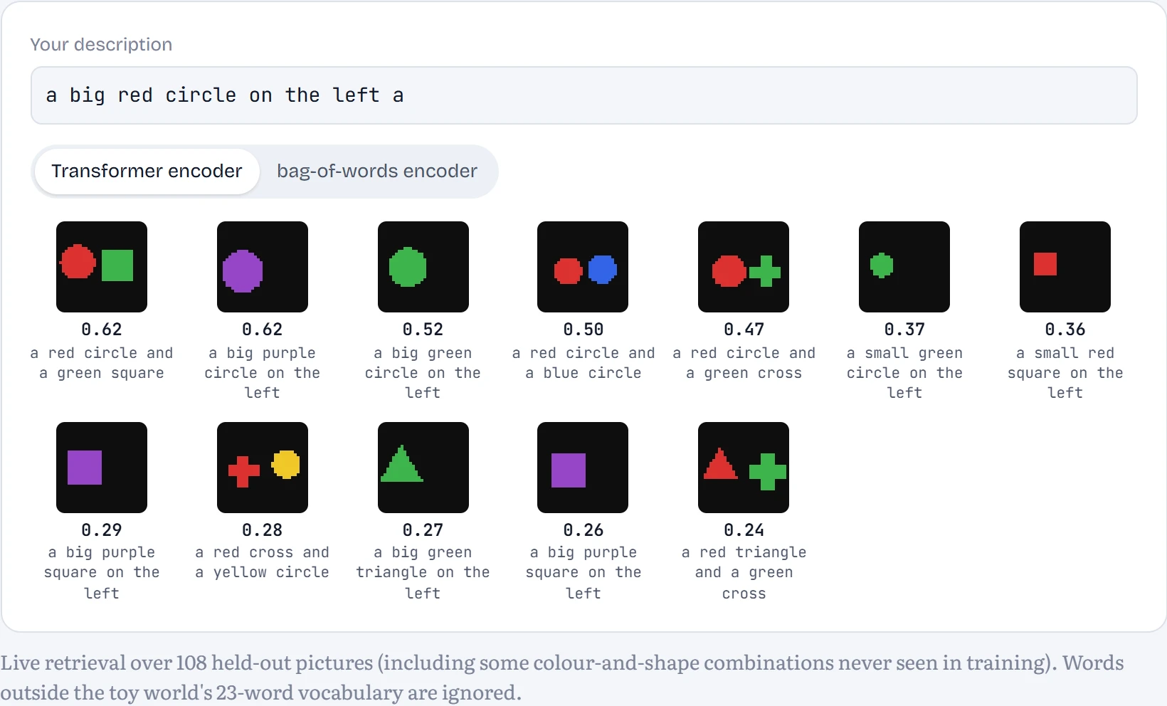
Now the experiment that makes CLIP interesting. I removed two colour-and-shape combinations, green triangles and purple circles, from training entirely. The model saw green things and triangles, purple things and circles, just never together. Then I asked it to name pictures of them, choosing among all 20 colour-shape captions. It's called zero-shot classification, since no labelled example of the class was ever shown.
The result: on held-out combinations, the bag-of-words model scored 100%, the Transformer 100% and the Transformer with hard negatives 100%, against 100%, 100% and 100% on combinations they had seen. Random guessing would give 5%. So the models really did learn “green” and “triangle” as separate ideas and combined them on the spot, which is the property that lets real CLIP recognize things nobody labelled. In this world that's easy, because colour and shape are cleanly separate in both the pictures and the words.
Predict first. Show the model a picture of a red circle to the left of a blue square, and offer it two captions: “a red circle and a blue square” (true) and “a blue circle and a red square” (same words, colours swapped). How often does the bag-of-words text encoder, which averages the word vectors without regard to order, choose the right one?
- 50%, a coin flip
- About 75%
- Nearly always, it's an easy task
Answer. Exactly a coin flip, by construction: the two captions contain the same words, and an encoder that averages word vectors gives them identical vectors, so their scores tie. (Measured: 47.4%, where a tie counts as half.) It can tell you there's red, blue, a circle and a square in the picture, and has no way to say which colour belongs to which shape. This is called the binding problem.
A Transformer text encoder sees word order, so it could tell the two captions apart. Does it? Here are all three models side by side. The third one adds hard negatives, an idea from the NegCLIP paper (Yuksekgonul and colleagues, 2023): for every two-object caption in a batch, I also put its colour-swapped version in as an extra wrong answer, forcing the model to care about who has which colour.
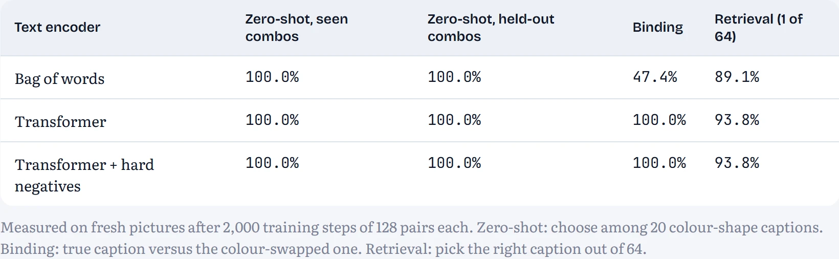
Look at the binding column, because it surprised me. I expected the plain Transformer to behave like a bag of words, as real CLIP famously does, and to need the hard negatives. Instead it reached 100.0% on its own, and the hard negatives had nothing left to add (100.0%). The reason is the size of this world. With 5 colours and 4 shapes there are only about 320 possible two-object captions, and each has 3 rivals with exactly the same words in a different arrangement. In a batch of 128, roughly 64 pictures have two objects, so the chance that a given caption's rival is sitting in the same batch is about 45%. The batch is full of natural hard negatives, and the only way to beat them is to bind each colour to its shape. The bag-of-words model can't, which is why its training loss stayed higher.
Now scale that up. Web captions describe millions of different things, so in a batch of real image–caption pairs, the chance that two captions differ only in who-does-what-to-whom is close to zero. Nothing in the loss rewards understanding word order, so the model doesn't bother. Our toy world is the exception that proves the rule: contrastive models learn exactly the distinctions their batches force them to make. That's the whole idea behind hard negatives: when the data doesn't supply the close calls, you add them deliberately.
Real CLIP shows the same weakness at scale: Yuksekgonul and colleagues found that it often can't distinguish “the horse is eating the grass” from “the grass is eating the horse”, and benchmarks like Winoground were built to measure it. In the lesson's search, the bag-of-words encoder ranks a red circle and a blue square exactly as it ranks a blue circle and a red square . The real CLIP was trained on 400 million image–caption pairs from the web with batches of 32,768, and its strength is breadth. It became the standard “eyes” for vision-language models and the text-understanding half of many image generators.
Giving a language model eyes
CLIP can match pictures with sentences, but it can't write one. For that you want a language model that can look. The recipe used by LLaVA (Liu and colleagues, 2023) and many open models since is surprisingly modular, and it's three parts:
An image encoder, usually a CLIP-trained ViT, turns the picture into a grid of vectors. A small projector, often just one or two linear layers, translates those vectors into the language model's embedding space, so they look like word embeddings. Then the language model reads them as if they were the first few “words” of the prompt, followed by the text. Nothing about the language model's architecture changes; it just gets some extra tokens that happen to come from a picture.
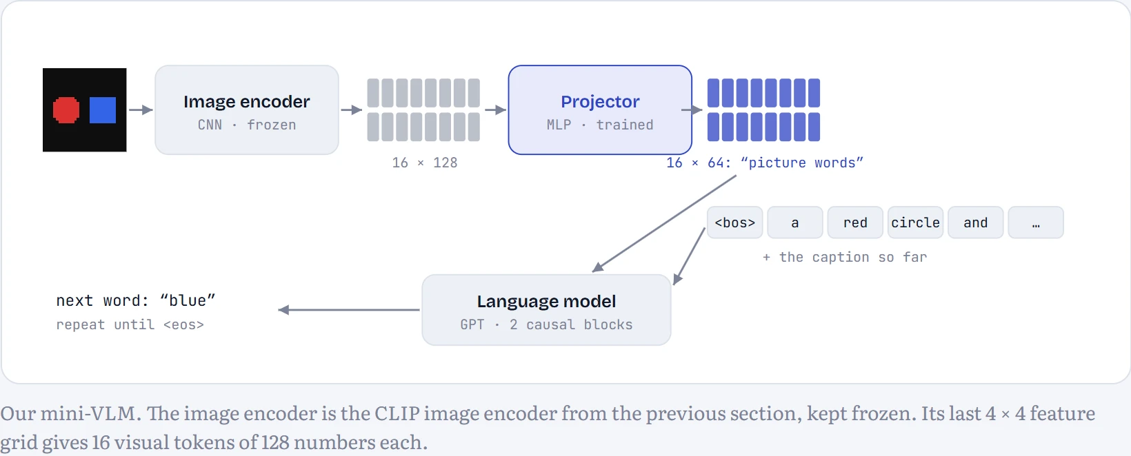
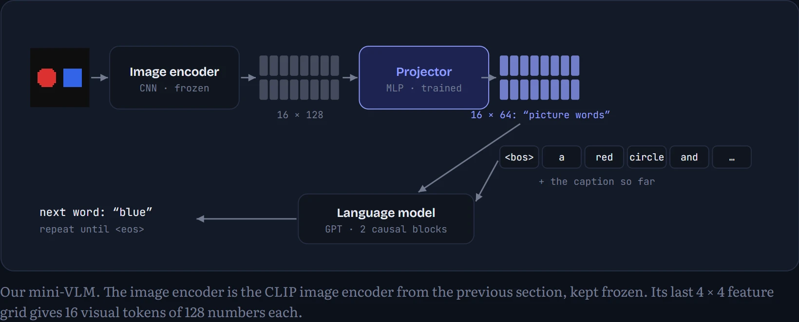
I trained ours in the same three stages LLaVA uses. Stage 0: train the language model (a 2-layer GPT) on captions alone, with no picture at all, so it learns the grammar of captions but has to guess what's in the image. Stage 1: freeze the language model and train only the projector: the language model already knows how to write captions, and the projector must learn to give it the right hints. Stage 2: unfreeze the language model and train everything together. How to read the table: each row is the model after that stage, judged on 600 fresh pictures by checking whether its caption names each attribute correctly. “Exact” means the whole caption is word-for-word right.
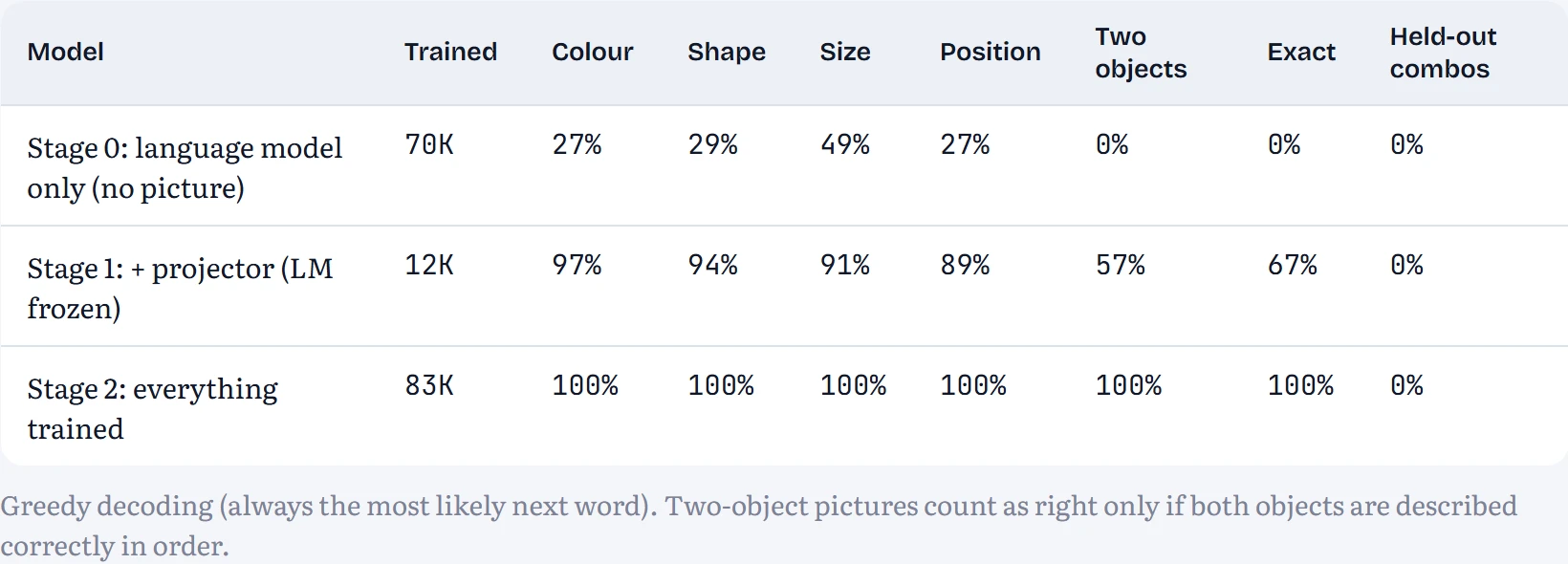
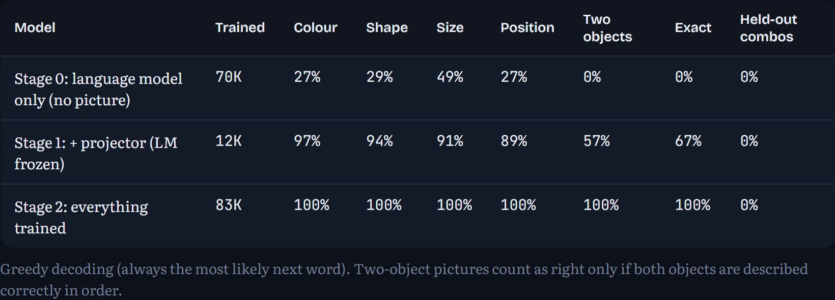
With its eyes shut, the stage 0 model writes perfectly formed captions and gets the colour right 27% of the time, about the 20% you'd expect from guessing one of five colours. That's the language model's prior: fluent, confident, and unrelated to the picture. Training only the projector, 12K numbers, while the language model stayed frozen, took colour accuracy to 97% and shape to 94%. A frozen language model can be steered into describing pictures purely by learning what to feed it. Unfreezing everything brought exact captions to 100%.
Then the held-out column, which is the most interesting number in the table. On pictures of green triangles and purple circles, the fully trained captioner named both colour and shape correctly 0% of the time. Remember that CLIP, trained on exactly the same pictures, picked the right caption for these combinations 100% of the time. The difference is generating versus choosing. CLIP only has to score a caption you hand it, and scoring “green” and “triangle” separately works fine. The captioner has to write the words, and its language model has learned, from thousands of training captions, that “green” is never followed by “triangle”. That learned habit outvotes the eyes every time, so it writes a familiar combination instead. It's hallucination in its purest form: a fluent, confident description shaped by what usually comes next rather than by what's in the picture.
Build a scene and the mini-VLM will describe it, running in your browser: the picture goes through the CNN encoder, the projector and the language model, one word at a time. How to read it: under each generated word is the probability the model gave it; low numbers mean it was unsure.
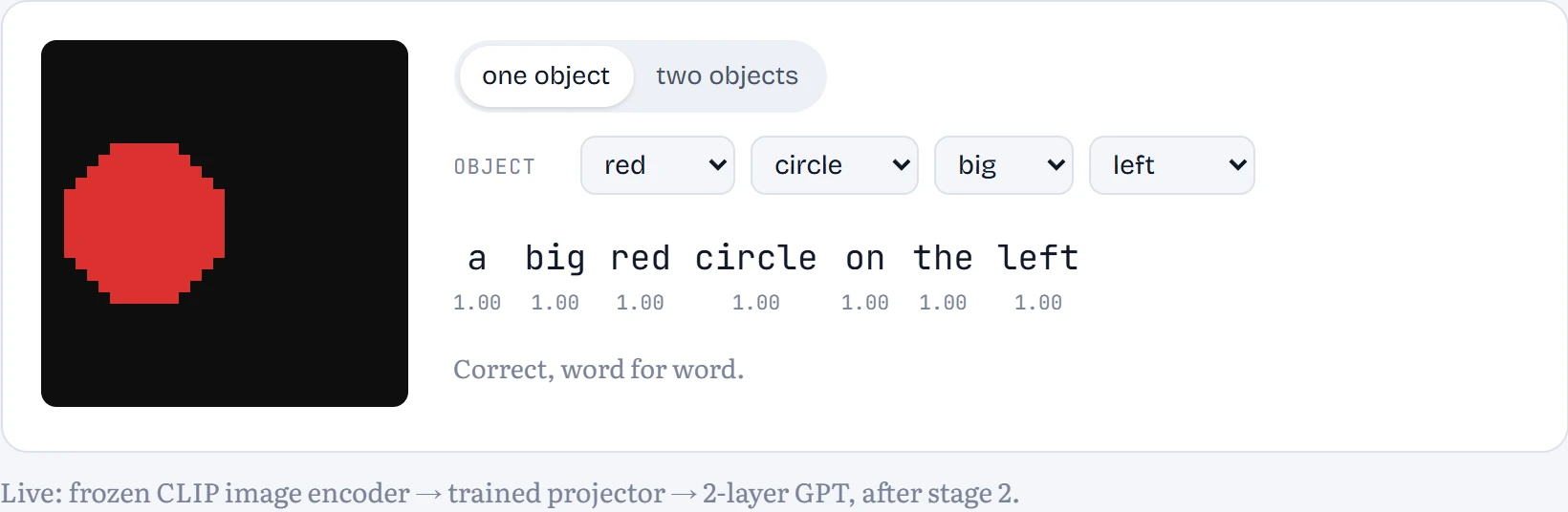
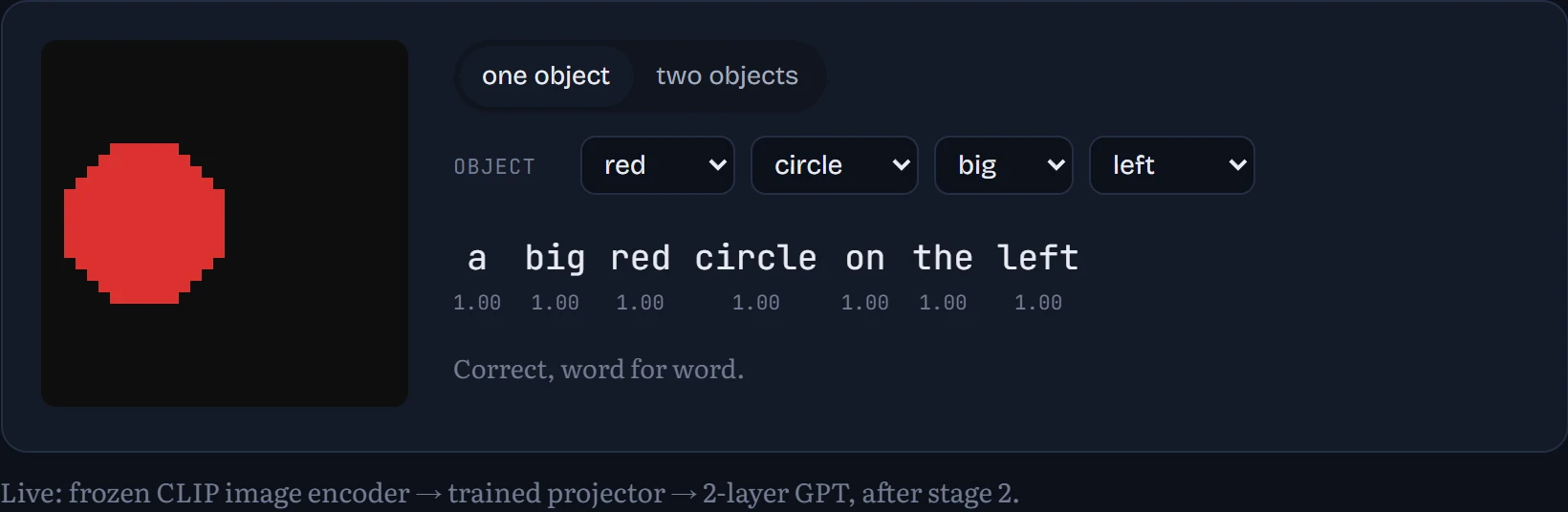
Real systems scale this up enormously, with the image encoder producing hundreds of tokens per image, and the language model having billions of parameters, but the wiring is the same. Its weakness is also the same: the language model is very good at writing plausible captions, so when the visual signal is weak it fills gaps with what's typical rather than what's there. That's object hallucination, and it's why a VLM may confidently describe a fork next to a plate that has none. Our stage 0 row is the extreme version: perfectly fluent captions, with eyes shut.
The newer alternative is native multimodality: instead of bolting a separately trained encoder onto a finished language model, the image is turned into tokens (with a learned image tokenizer, or as patches), and a single model is trained on interleaved text and image tokens from the start. Meta's Chameleon is a published example; several frontier models are believed to work this way, though their details are not public. A natively multimodal model can also output image tokens, so the same network that reads pictures can draw them.
Hearing: from air pressure to text
Sound is a list of numbers too: a microphone measures air pressure thousands of times a second. At 8,000 measurements per second (telephone quality), one second of speech is 8,000 numbers, and a single vowel spans thousands of them. Feeding raw pressure values to a model works, but it's wasteful, so almost every speech system first converts sound into a picture of which pitches are present when: a spectrogram.
To make this lesson's speech experiments fully transparent, I didn't use recordings. I wrote a small voice synthesizer that works the way your own voice does. Your vocal folds buzz at a steady rate (that's the pitch, around 100 to 250 buzzes a second), producing a sound rich in all its harmonics. Your mouth and throat then act like a set of resonating tubes, boosting a few frequency bands and damping the rest. Those boosted bands are called formants, and their positions are what make an “ee” sound different from an “oo”: it's the shape of your mouth, not your vocal folds, that changes between vowels.
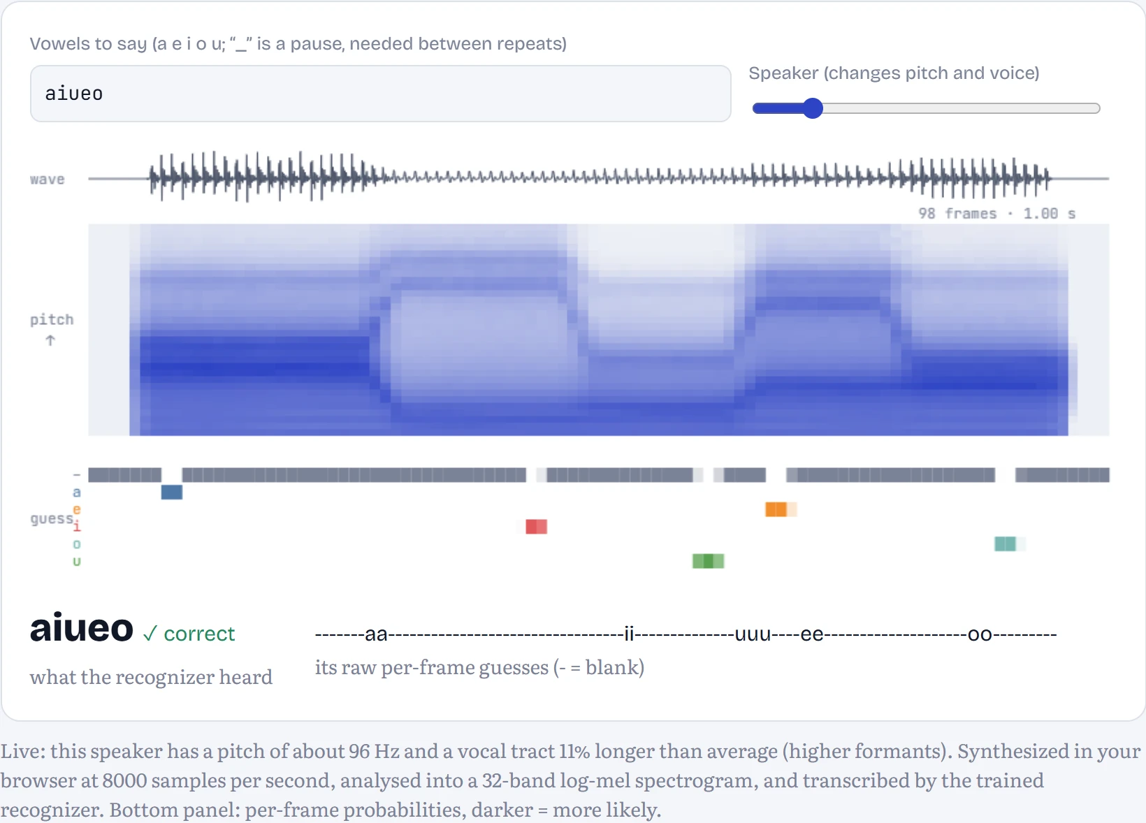
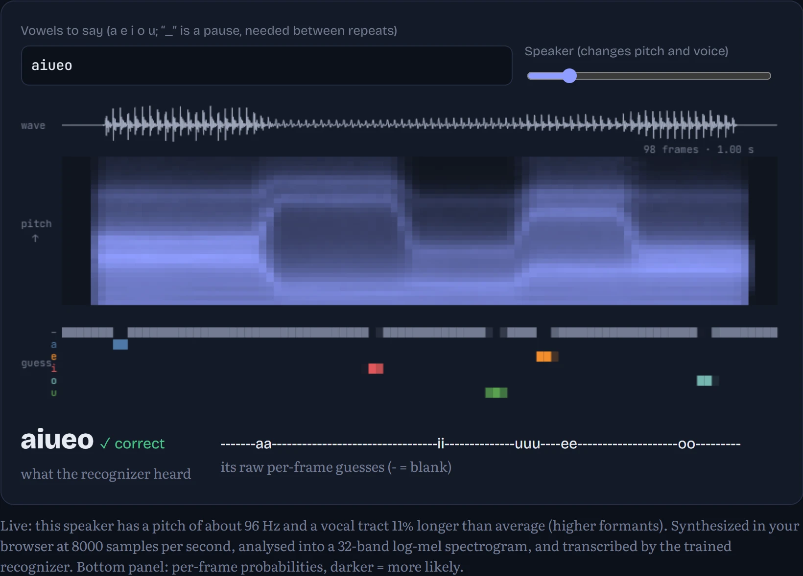
How to read it: the top strip is the raw waveform, the air pressure over time. The middle panel is the spectrogram: time runs left to right in 10-millisecond steps, pitch runs bottom (low) to top (high), and brighter means more energy. Each vowel shows as a block with its own pattern of bright bands; those bands are the formants. The frequency axis uses the mel scale, which squeezes high frequencies together the way human hearing does (we notice a 100 Hz change at low pitch far more than at high pitch). The bottom panel shows what the recognizer thinks at every 10-millisecond step, which brings us to the clever part.
CTC: how to train without knowing where each sound is
Our training data says “this clip is a i u”. It doesn't say which milliseconds belong to which vowel, and in real speech nobody labels that either. The model makes one guess per 10-millisecond frame, so there are about a hundred guesses for three letters. How do you compute a loss? CTC (connectionist temporal classification, Graves and colleagues, 2006) solves this with one extra symbol, the blank, meaning “nothing new here”. Any frame-by-frame sequence of guesses is turned into text by two rules: merge repeated symbols, then delete blanks. So – – a a a – – i i – u – reads as “aiu”. The CTC loss adds up the probability of every frame sequence that reads as the right answer (there are astronomically many, but a dynamic-programming trick sums them efficiently) and maximizes that total.
The blank also solves a subtle problem: how do you say the same vowel twice? “aa” collapses to “a”, so a doubled vowel needs a blank between: a a – a a reads as “aa”. In our synthesizer, I put a short pause between repeated vowels for the same reason.
Predict first. A trained CTC model listens to a vowel that lasts 20 frames. What do you expect its per-frame guesses to look like during that vowel?
- The vowel on all 20 frames
- Mostly blank, with the vowel on just one or two frames
- A smooth mix of the vowel and blank
Answer. Mostly blank, with sharp spikes. In the fully trained model on the clip below, 87% of frames have “blank” as the top guess. CTC doesn't care where inside the vowel the label appears, only that the collapsed sequence comes out right, and the cheapest way to be confident about that is to say blank almost everywhere and fire each vowel once. These “peaky” outputs are a known signature of CTC models.
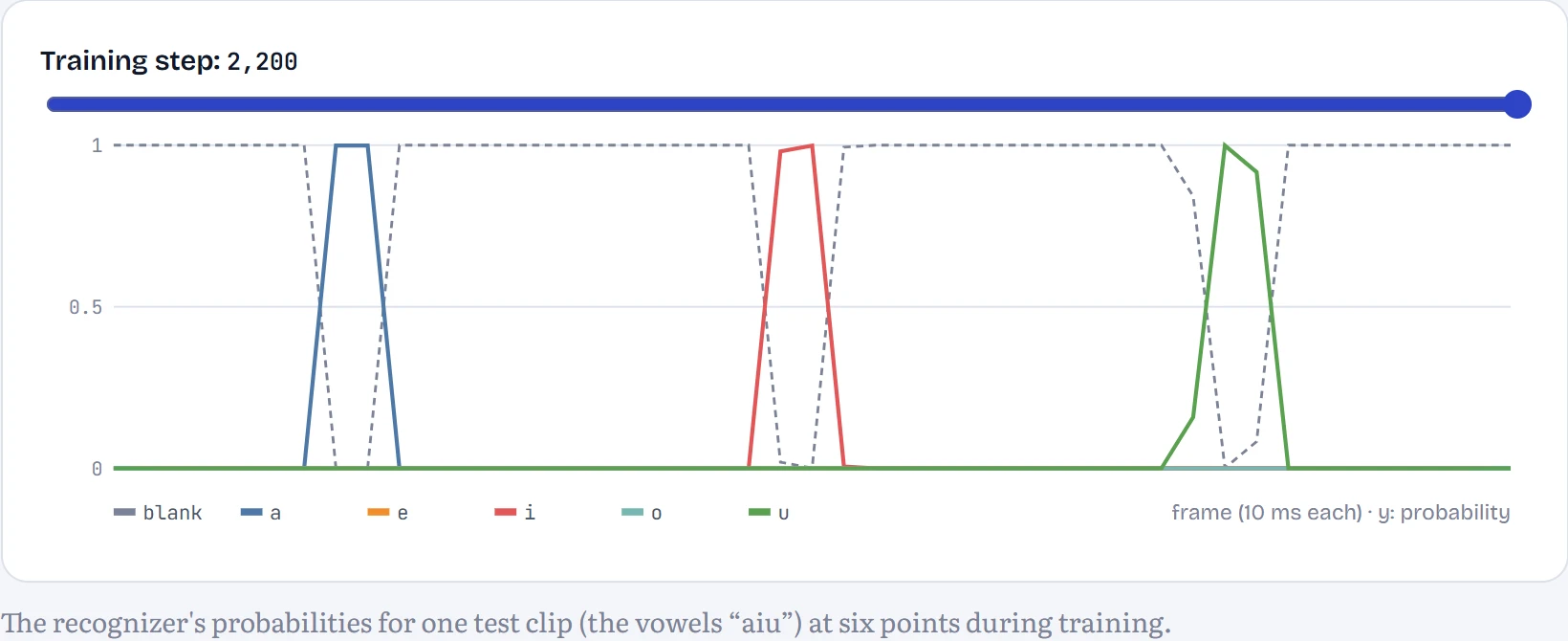
Our recognizer has 81,542 parameters: two 1-D convolutions that look at 5 frames at a time, then a bidirectional GRU (a recurrent network that reads the frames forwards and backwards, Chapter 8) and a final layer that scores the 6 symbols. I trained it on 6,000 synthesized clips of 2 to 7 vowels, each with a random speaker, for 12 passes, which took 27 minutes. For the first 2 passes, it got everything wrong: it had discovered that predicting blank on every frame is a cheap way to lower the loss early on, and sat there, outputting nothing. That's a common CTC phase. Then it broke through. On 400 fresh test clips, it ends with a character error rate of 0.0% (the edit distance between what it heard and the truth, divided by the length) and gets 100% of whole clips exactly right.
Then I tested it on a voice outside its training range: a pitch of 70 Hz (training speakers were 95 to 215 Hz) and a longer vocal tract, which shifts every formant down by 20%. Its error rate went from 0.0% to 14.2%. Nothing about the vowels changed; only the voice did, and the model had never learned that formants scale with the speaker. Real recognizers hit the same wall with accents, children's voices and unfamiliar microphones, which is why training data diversity matters so much.
Real speech systems
Real recognizers face everything our synthesizer leaves out: consonants, accents, background noise, overlapping talkers. OpenAI's Whisper (Radford and colleagues, 2022) shows how far the same ingredients go at scale. It turns 30-second windows of audio into an 80-band log-mel spectrogram, encodes it with a Transformer, and uses a second Transformer to write the transcript token by token, attending to the audio as it goes, the same encoder-decoder pattern as machine translation. It was trained on 680,000 hours of audio with existing transcripts from the web. Writing the text with a decoder instead of CTC lets it add punctuation and capitalization, and even translate, but makes it slower and occasionally lets it invent text during silence, a speech version of hallucination.
Going the other way, from text to speech, modern systems mostly use audio tokens. A neural audio codec, such as SoundStream or EnCodec, learns to compress audio into a short sequence of discrete codes (a few hundred per second) and decode them back with little audible loss. Once speech is tokens, a language model can generate it: text-to-speech becomes “predict the next audio token”, and a voice assistant can listen and speak in tokens without ever converting to text. Give such a model a few seconds of someone's voice as a prompt, and it continues in that voice. That's voice cloning, and it's why responsible releases require consent from the speaker, add inaudible watermarks to generated audio, and pair generators with detectors: a cloned voice on a phone call is a very effective scam.
Continue the lesson
The whole lesson, with its drawings and its questions. 8 more sections after the ones above.