
LLM inference: sampling strategies, prefill and decode, KV cache, quantization, speculative decoding and test-time compute
A language model writes one token at a time: output a probability for every next token, pick one, append it and run again. Inference is about two questions: which token to pick, from greedy decoding to temperature, top-k and top-p sampling, and how to make each turn of the loop cheap with the KV cache, quantization and speculative decoding.
What this page answers
What is the difference between top-k and top-p sampling?
Top-k keeps only the k most likely next tokens. Top-p keeps the smallest set of likely tokens whose probabilities add up to p. Either way the rest are ruled out and the kept probabilities are renormalized. Read it in “Choosing the next token”
What is the KV cache?
A store of each token's attention keys and values from earlier steps, so generating the next token computes them only for the new token instead of for the whole text again. Read it in “Prefill, decode and the KV cache”
One token at a time
A language model never writes a sentence. It does one thing: given the text so far, output a probability for every possible next token. Generation is a loop around that. Pick a token from the distribution, append it, run the model again, and repeat until you hit a stop token or a length limit. Everything in this chapter is about two questions that loop raises: which token do you pick, and how do you make each turn of the loop cheap?
Here's the loop running live on the story model from Chapter 11 (4 Transformer blocks, character level). How to read it: the bars show the model's probabilities for the next character, after the settings below are applied: grey bars are characters the current rule has ruled out, and the remaining blue bars are renormalized to add up to 1. Each generated character is shaded by the probability it had when it was picked, so pale characters were long shots.
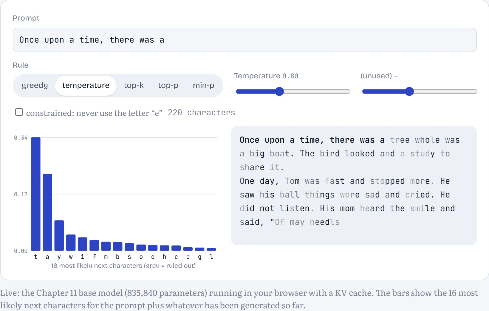
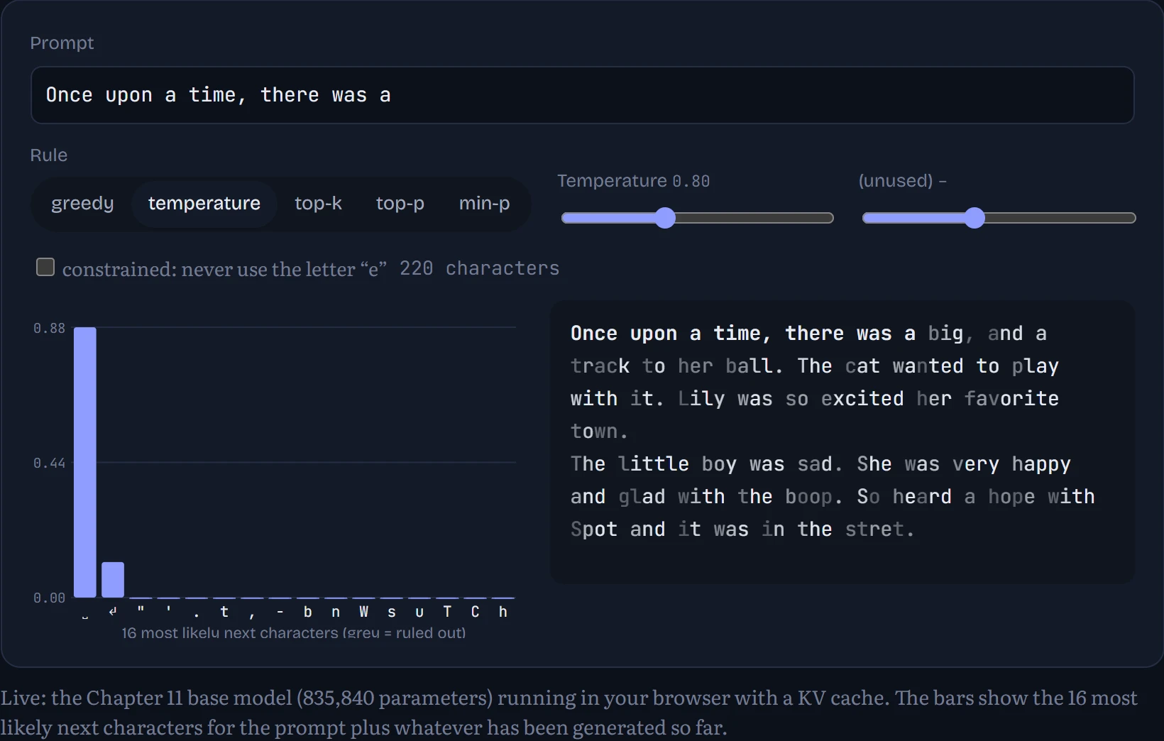
Choosing the next token
The obvious rule is greedy: always take the most likely token. It's deterministic and often fine for short factual answers, but on open-ended text it gets stuck, because the most likely continuation of a phrase is often a phrase it just wrote. Beam search keeps the few most probable whole sequences instead of one, which works well for translation, where there's one right answer, and badly for stories, where it amplifies the same blandness. The alternative is to sample: pick tokens at random in proportion to their probabilities, which brings variety and occasional nonsense.
The other rules tame sampling. Temperature divides every logit by T before the softmax: T below 1 sharpens the distribution towards the favourites, T above 1 flattens it towards uniform. Top-k keeps only the k most likely tokens. Top-p, or nucleus sampling (Holtzman and colleagues, 2019), keeps the smallest set of tokens whose probabilities add up to p, so the set is small when the model is sure and large when it isn't. Min-p (Nguyen and colleagues, 2024) keeps every token whose probability is at least some fraction of the top token's, which scales the cut with the model's confidence.
Predict first. I generated stories with each rule and counted three things: how often the model repeats itself, how many of its words are real English words, and how different the stories are from one another. Which rule gave the least variety between stories?
- Temperature 1.6
- Beam search
- Top-p 0.9
Answer. Beam search. Only 38% of its word triples were unique across stories, and 10% of the triples within each story were repeats: it finds the single most probable path, which for stories means the same safe phrases again and again. Greedy decoding is similar (70% unique).
How to read the chart: each dot is one decoding rule. Further right means more variety between stories (the share of word triples that appear only once across all of them); higher means more of the generated words are real words from the training text. The ideal is the top-right corner: varied and coherent.
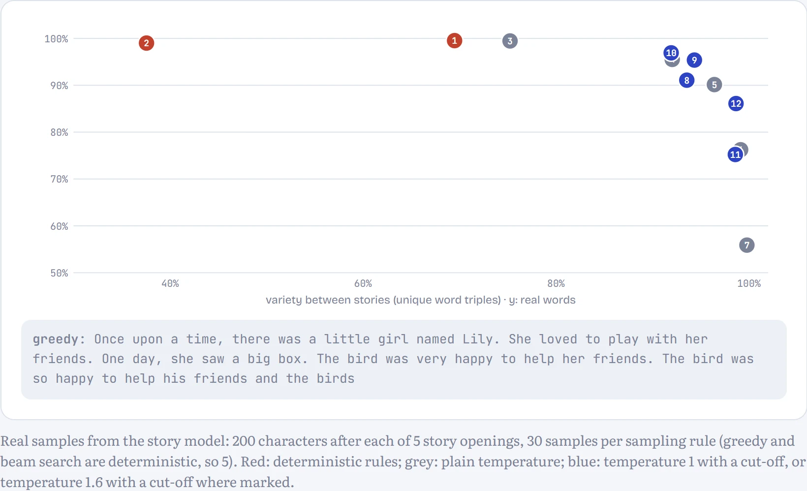
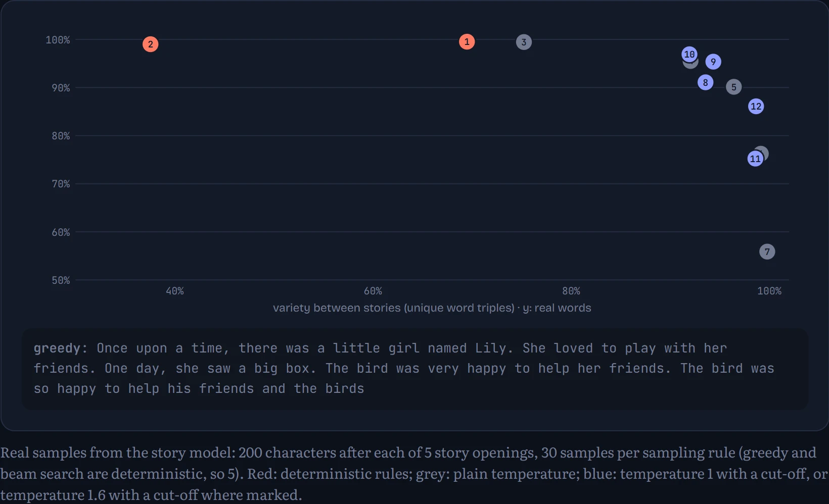
The chart shows the trade-off sampling is about. Raising the temperature walks you to the right (more variety) and down (more invented words): at T = 1.6, 56% of words are real, and you can see why in the sample. A cut-off pulls the high-temperature points back up. At T = 1.6, top-p 0.9 kept 75% real words, and min-p 0.1 kept 86% with almost the same variety, which is the case its authors make for it: the cut scales with how confident the model is, so the long tail of junk characters gets cut harder when the model is sure of the next letter. At normal temperature, top-p 0.9 (95% real words) beats plain sampling (90%) at a small cost in variety. In practice most chat products sample at a temperature somewhere around 0.7 to 1 with a top-p or min-p cut-off.
Constrained decoding is the same machinery used to enforce rules. Before sampling, set the probability of every forbidden token to zero. Forbid the letter “e” and the model never writes one: it isn't trying to avoid the letter, it simply can't pick it, so it routes around it. Production systems use the same trick to guarantee valid JSON or match a schema, by allowing only the tokens a grammar permits at each step. And a footnote on nondeterminism: even at temperature 0, large deployed models often don't give identical answers to identical prompts. Floating-point addition isn't associative ((0.1 + 0.2) + 0.3 = 0.6000000000000001, but 0.1 + (0.2 + 0.3) = 0.6, computed by your browser just now), and on a GPU the order of additions changes with how requests are batched together, which can flip a near-tie between two tokens. One flipped token changes everything after it.
Prefill, decode and the KV cache
Generation has two very different phases. Prefill reads your whole prompt in one forward pass: every position is processed in parallel, as in training, so the hardware is kept busy. Decode then produces one token per forward pass, and each pass does very little arithmetic per byte of weights it has to read from memory. That's the memory wall from Chapter 10: decode is limited by memory bandwidth, not by arithmetic.
The KV cache keeps decode from being even worse. Attention at step t needs the keys and values of every earlier token. Without a cache you'd recompute them all at every step, so the cost of each new token grows with the length so far; with one, you compute the new token's key and value once, store them, and reuse them forever. How to read the charts: left, total time to generate 250 characters with and without the cache, on a laptop CPU; right, how many tokens per second each phase processes.
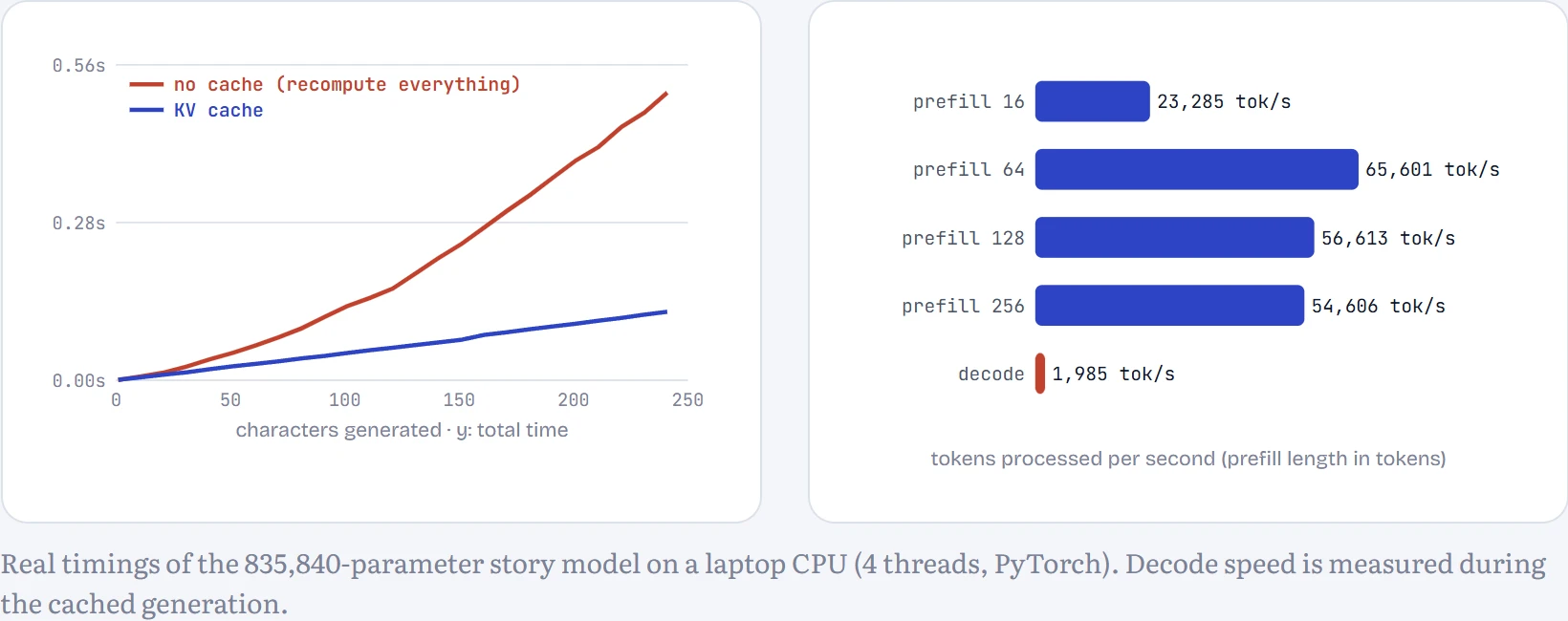
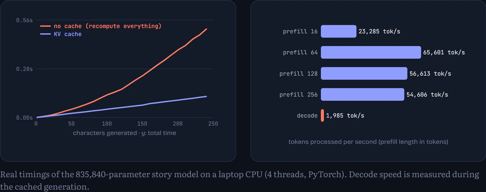
Without the cache, generating 250 characters took 0.51 s, and the curve bends upward because each new character recomputes everything before it. With the cache it took 0.12 s, a straight line: 4.2× faster, and the gap keeps widening with length. On the right, the two phases: prefill processed up to 65,601 tokens per second, decode 1,985, about 33× slower per token on the same machine and model. On GPUs serving big models the gap is similar in spirit. That's why time-to-first-token (prefill) and time-per-output-token (decode) are measured separately, and why output tokens cost more.
Serving systems are built around these facts. Because decode is memory-bound, the cheapest way to get more throughput is to decode many requests at once: reading the weights once serves the whole batch. Continuous batching (Orca, Yu and colleagues, 2022) adds a new request to the batch the moment another finishes, instead of waiting for the slowest request in a fixed batch. PagedAttention (vLLM, Kwon and colleagues, 2023) stores each request's KV cache in small fixed-size blocks, like an operating system's memory pages, so caches of unpredictable length don't waste memory on reserved space. Together they're why one GPU can serve dozens of simultaneous conversations.
Quantization: fewer bits per weight
If decode spends its time reading weights, make the weights smaller. Quantization stores each weight with fewer bits. The simplest version: for each row of a weight matrix, find the largest absolute value, divide the range from minus that to plus that into evenly spaced levels (255 levels for 8 bits, 15 for 4 bits), and round every weight to the nearest level. Store the small integers plus one scale number per row. Grouping uses a separate scale for every 32 weights, so one large weight doesn't stretch the grid for its whole row.
How to read it: the histogram shows the real weights of one layer of the story model; the vertical lines are the levels a weight can be rounded to at the chosen bit width (for the row containing the largest weight). The fewer the bits, the coarser the grid. The table shows what each format does to the model's loss on held-out stories.
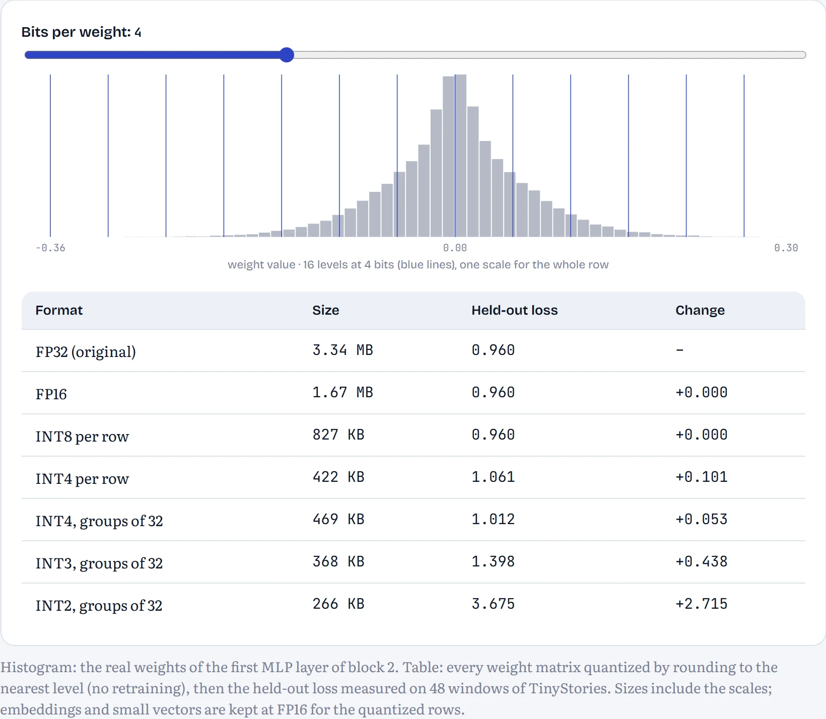
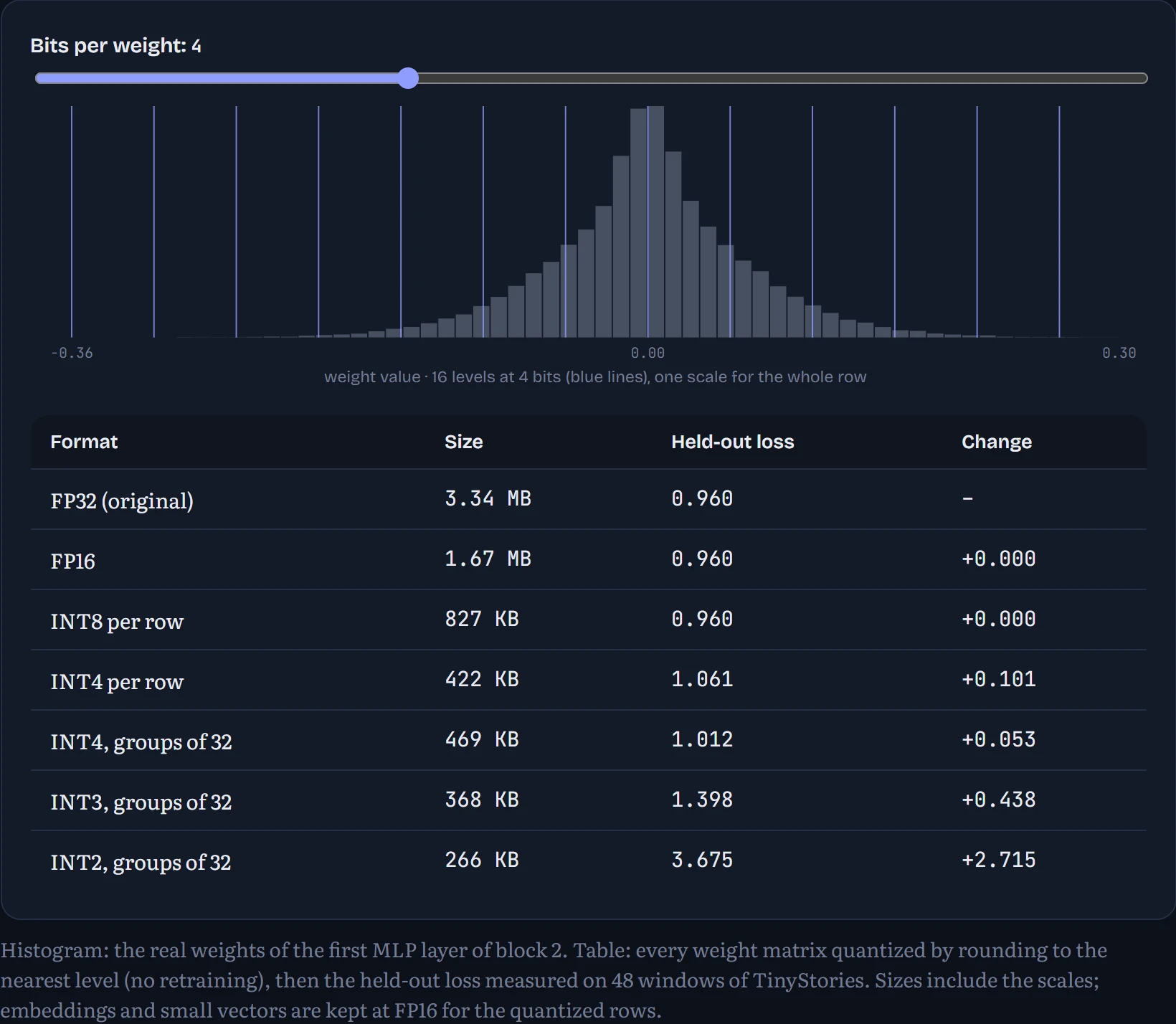
Eight bits is essentially free: loss 0.960 becomes 0.960, at a quarter of the original size. Four bits starts to cost: 1.061 with one scale per row, but 1.012 with a scale per group of 32 weights, which recovers most of the damage for 10% more space. Look at the histogram to see why grouping helps: most weights crowd near zero, and a single large weight sets the grid spacing for its whole row, wasting most of the 16 levels on empty space. Three bits hurts (1.40), and two bits destroys the model (3.67, worse than knowing nothing about the story). Real 4-bit methods such as GPTQ and AWQ do better than plain rounding by adjusting weights to compensate for each other's rounding errors, which is how people run 70-billion-parameter models on a single consumer GPU.
Speculative decoding: guess fast, check in bulk
Here's a neat consequence of prefill being cheap and decode being expensive. Checking five tokens costs a big model about the same as generating one, because checking is a parallel pass over all five. So let a small, fast draft model guess the next few tokens, then run the big model once over all of them. Accept the guesses the big model agrees with, and at the first disagreement take the big model's own choice instead. With the right acceptance rule (Leviathan and colleagues; Chen and colleagues, both 2023), the output has exactly the same distribution as sampling from the big model alone: you only get speed, never different answers.
I trained a draft model for the story model: one Transformer block instead of four, 64-number vectors instead of 128, 71,360 parameters (about 12 times smaller), trained for a few minutes. Its held-out loss is 1.29, far worse than the big model's, so it's often wrong. Does that matter? How to read the chart: for each number of drafted tokens γ, how many tokens of finished text each call to the big model produces (higher is better; normal decoding is exactly 1), and, after the dot, the share of drafted tokens the big model accepted.
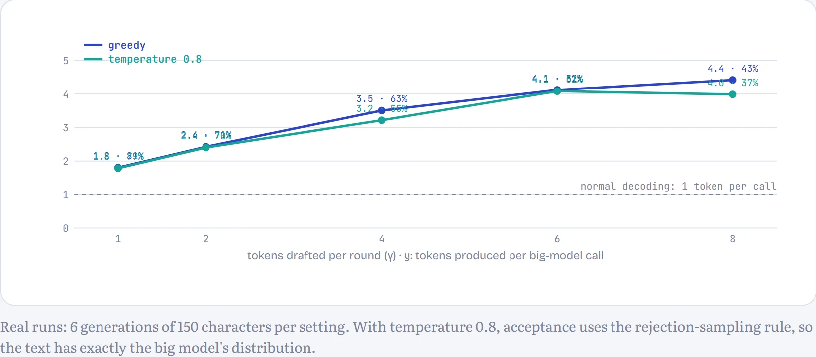
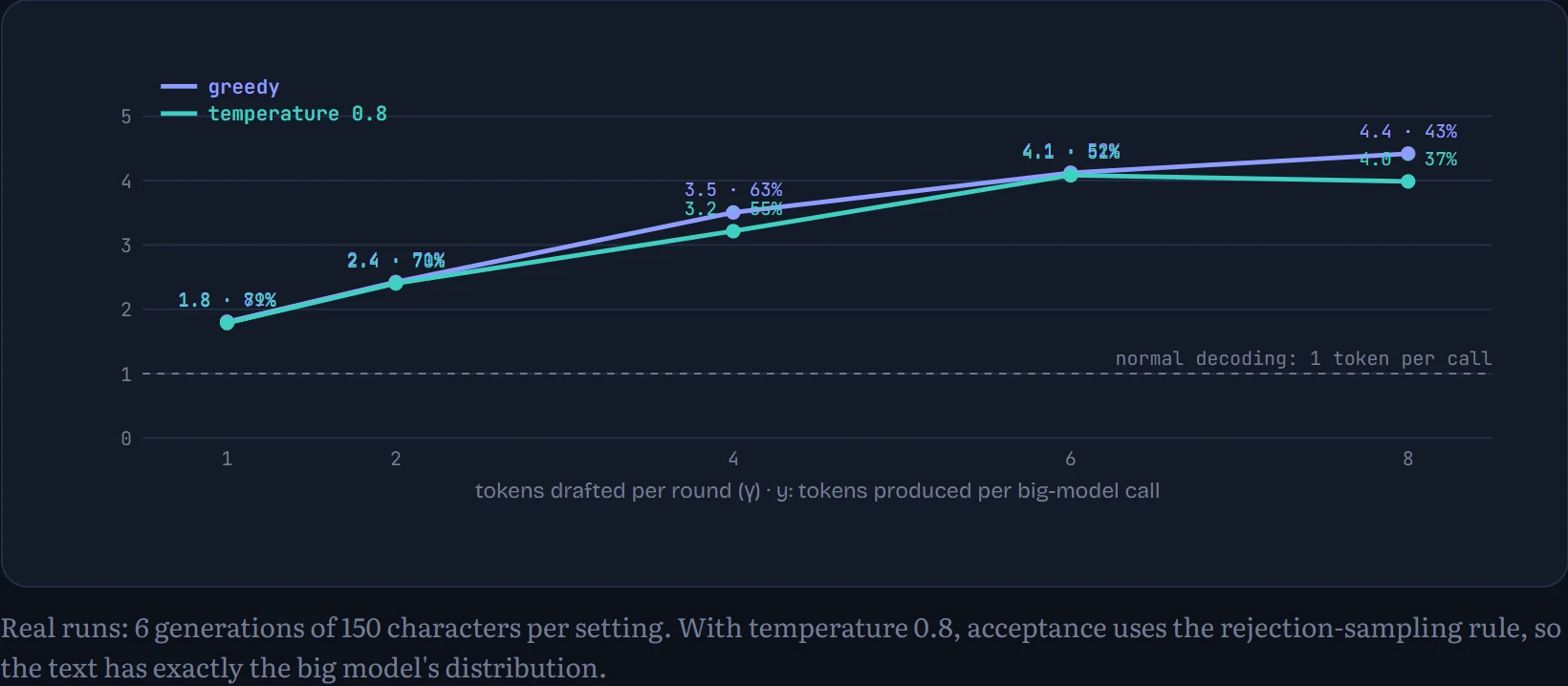
Even this weak draft makes each big-model call produce several tokens: 3.5 on average when drafting 4 at a time (greedy), up to 4.4 at γ = 8. Character-level stories are full of predictable stretches (“nce upon a time” after “O”) that a tiny model gets right, so the big model can rubber-stamp them in bulk. Acceptance falls as γ grows, because each extra guess is conditioned on all the earlier ones being right, so the benefit levels off, and with sampling it even dips at γ = 8. Whether this saves wall-clock time depends on hardware: on a GPU, where a big-model call over 5 tokens costs about the same as over 1, the speed-up is nearly the tokens-per-call figure (minus the draft's own cost). On our laptop CPU, with a model this small, it barely matters; for a 70-billion-parameter model on a GPU, speed-ups of 2 to 3× are typical.
Context: what the model can see
Everything the model knows about your request is in its context window. More context helps: the further into a document the model is, the more it knows about the characters, the topic and the style. You can see it directly by measuring the loss at every position. How to read the chart: each point is the average loss (lower is better) of the story model at that position of its 256-character window, over 300 held-out windows. Position 0 has no context at all.
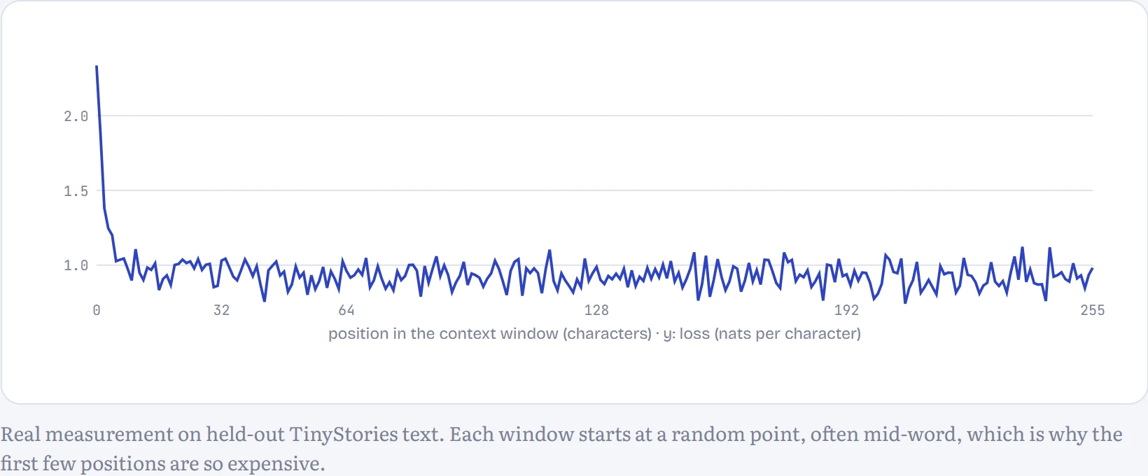
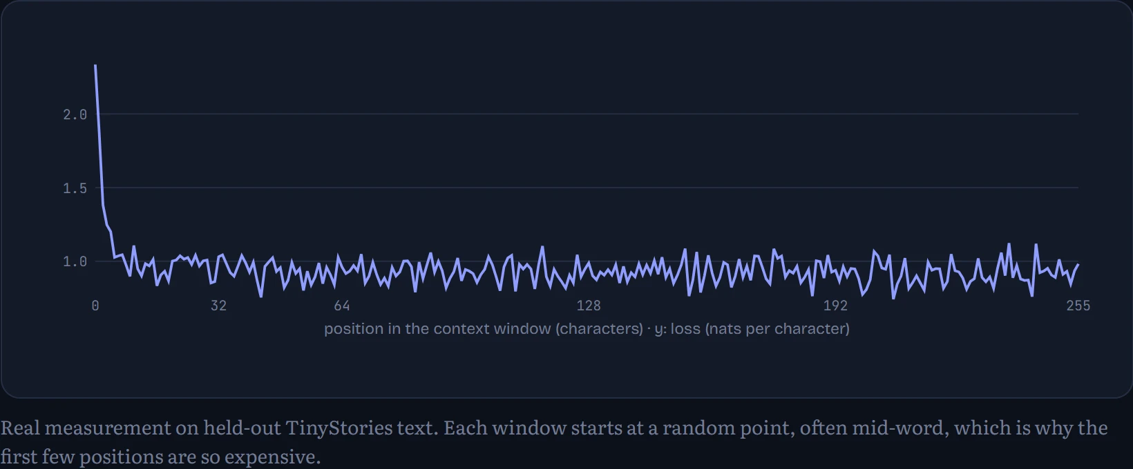
At position 0 the model is guessing blind: 2.34 nats. Within a few characters it can see the current word and the loss halves. After that the gains get small: 0.974 averaged over positions 8–15, 0.928 over 30–60, and 0.918 over 200–255. So this small model gets most of its benefit from the last few dozen characters and only a little more from the rest of the window. That's an honest picture of a small model trained briefly: it has learned to use local context well and distant context only slightly, the same reason Chapter 15 found no induction heads in it. Large models keep improving over much longer spans, using a character's name from three pages back or a definition from the start of a document, which is what makes long context windows worth the engineering.
Stretching a model past its training length, measured
Here are three of those long-context techniques tested for real. I trained small Transformers on 64-character windows and then asked them to read 256 characters, four times further than they'd ever seen (Chapter 9.2 has the full comparison of position schemes). How to read the chart: the average loss at positions beyond the training length (lower is better); the dashed line is how well the same RoPE model does inside its training length.
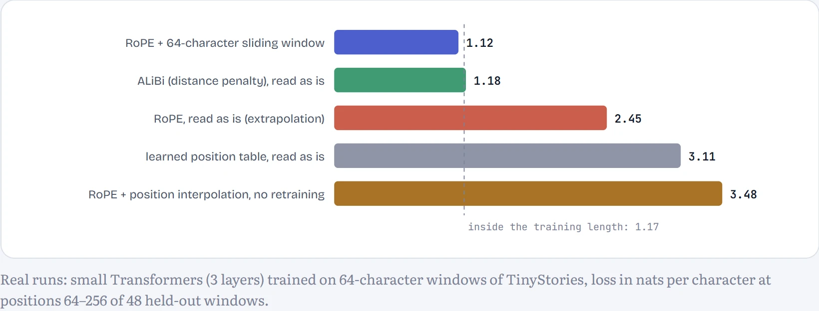
Read as is, the RoPE model gets steadily worse past its training length (2.45, against 1.17 inside it). A sliding window fixes that completely (1.12): if every token only ever looks 64 positions back, every distance it meets is one it trained on. The price is that nothing further back can be seen at all, which is why models such as Mistral and Gemma mix sliding-window layers with a few full-attention layers. ALiBi, whose distance penalty fades out far tokens on its own, extrapolates almost for free (1.18). Position interpolation made things worse without retraining (3.48): squeezing the positions changes every distance the model knows, so in practice it's always followed by a short fine-tune at the longer length, and YaRN refines it by stretching only the slow-turning frequencies. None of these tricks makes the model use distant information well; that's the separate problem of lost-in-the-middle below.
Frontier models have context windows of hundreds of thousands to millions of tokens, which takes several tricks at once. Position schemes that extrapolate, such as RoPE (Chapter 9) with frequency scaling methods like YaRN, let a model trained on shorter sequences handle longer ones after a little extra training. FlashAttention (Chapter 8) avoids storing the full attention matrix, and attention can be split across many GPUs (ring attention). Some models use sliding-window attention in most layers, so only a few layers see everything. Long context also has a known weakness: models use information at the beginning and end of a long prompt better than information buried in the middle (“Lost in the Middle”, Liu and colleagues, 2023), although newer models have narrowed the gap.
Long prompts are expensive to prefill, and many prompts share a long beginning: the same system prompt, the same document, the same conversation so far. Prompt caching keeps the KV cache of a shared prefix and reuses it. On our story model, answering 20 questions that share a 200-character prefix meant processing 4,400 tokens without caching and 600 with it (the prefix once, plus 20 new characters per question), and took 0.139 s against 0.080 s on the CPU. The time saving is smaller than the token saving because a model this small spends much of its time on per-call overhead; for a large model, where prefill compute dominates, the time saving approaches the token saving. Hosted APIs pass this on as a large discount for cached input tokens.
OPEN RESEARCH. How does in-context learning work? Part of the answer is the induction heads you dissected in Chapter 15, which copy patterns from earlier in the context. Researchers have also found that large models can implement something like learning algorithms inside a forward pass, and that a prompt's examples are compressed into “task vectors” that can be transplanted into other prompts. How much of in-context learning is retrieving skills learned during training, versus genuinely learning something new from the prompt, is still debated.
Continue the lesson
The whole lesson, with its drawings and its questions. 6 more sections after the ones above.