
Evaluation and mechanistic interpretability: bootstrap confidence, logit lens, probes, induction heads and sparse autoencoders
You know a model is good by testing it on questions it has not seen and counting, but benchmark questions leak onto the web and into training data. Interpretability reads the model from inside: the logit lens shows its guess at every layer, probes test what it knows, and sparse autoencoders untangle features held in superposition.
What this page answers
What is benchmark contamination?
When a model has seen a benchmark's questions, and often its answers, during training because they were copied across the web. It inflates the score and is very hard to rule out. Read it in “How do you know a model is good?”
What is the logit lens?
Apply the model's final LayerNorm and unembedding early, after any block, to see what it would predict if it had to answer right now. Read it in “Reading the model as it thinks: the logit lens”
How do you know a model is good?
The honest answer is: you test it on questions it hasn't seen, and you count. A benchmark is just a fixed set of questions with known answers, kept away from training, so everyone can compare models on the same exam. MMLU (multiple-choice questions across 57 school and professional subjects), GSM8K (grade-school maths word problems), HumanEval and SWE-bench (writing code that passes tests) are household names in the field.
The whole idea rests on one assumption: the model has never seen the exam. On the modern web that's a fragile assumption. Benchmarks get published, quoted, discussed and copied into thousands of pages, and a model trained on a large slice of the internet may well have read the questions, and the answers. That's called contamination, and it's very hard to rule out, because nobody can read a trillion tokens of training data to check.
So I contaminated models on purpose, to see what it does to the score. The task: two-digit multiplication, like 47*83=3901, which a small Transformer learns slowly and imperfectly. I built a benchmark of 1,000 problems and trained two identical small models on random multiplication problems that never overlap the benchmark. One difference: for the second model, 5% of its training lines were drawn from half of the benchmark (500 “leaked” questions). It never saw the other 500. I also kept 1,000 fresh problems that appear nowhere. Then I repeated the experiment with a much heavier leak (25% of training lines), and with the 3-digit addition task from Chapter 11.
Predict first. The leaky model learns multiplication from mostly honest data, but has seen half the exam questions many times. Compared with the clean model, what happens to its score on the 1,000 fresh problems?
- Higher: practising the exam helped it learn
- About the same, give or take noise
- Much higher: it has seen half the answers
Answer. About the same, give or take noise. On the 1,000 fresh problems, the 5%-leak model scores 23.1% and the 25%-leak model 36.5%, against 32.1% for the clean model: one lower, one higher, with no consistent direction. At this stage of training, separately trained models differ by several points just by chance. What doesn't vary is the gap inside each leaky model between questions it saw and questions it didn't. Seeing exam questions made them better at those questions, which is the definition of memorizing, not better at multiplication.
Here's what happened over training. How to read it: each line is accuracy (share of problems answered exactly right) against training steps. Solid lines are the leaky model; the clean model's benchmark score is the dashed grey line. Watch the gap between the leaky model's leaked questions (red) and everything else.
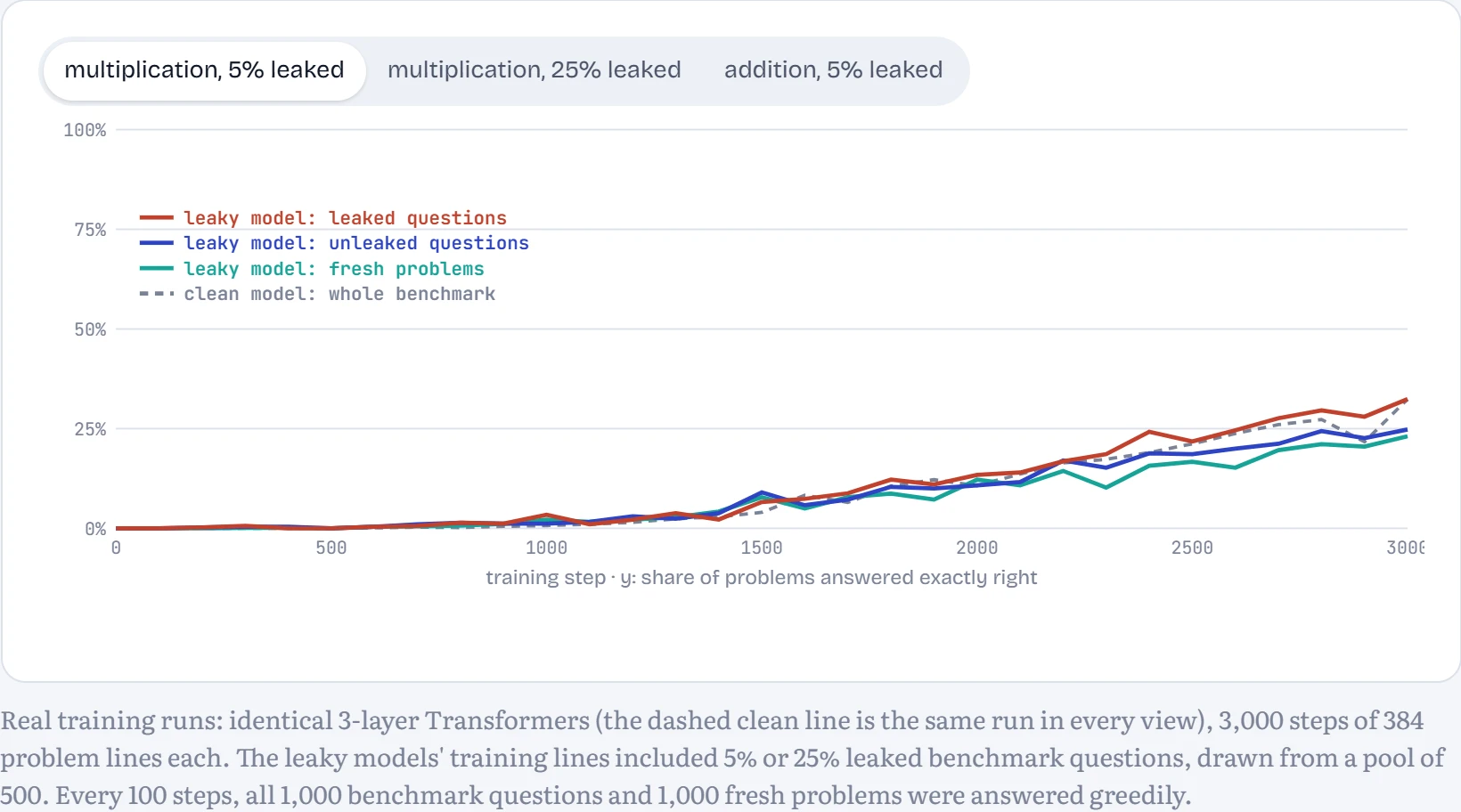
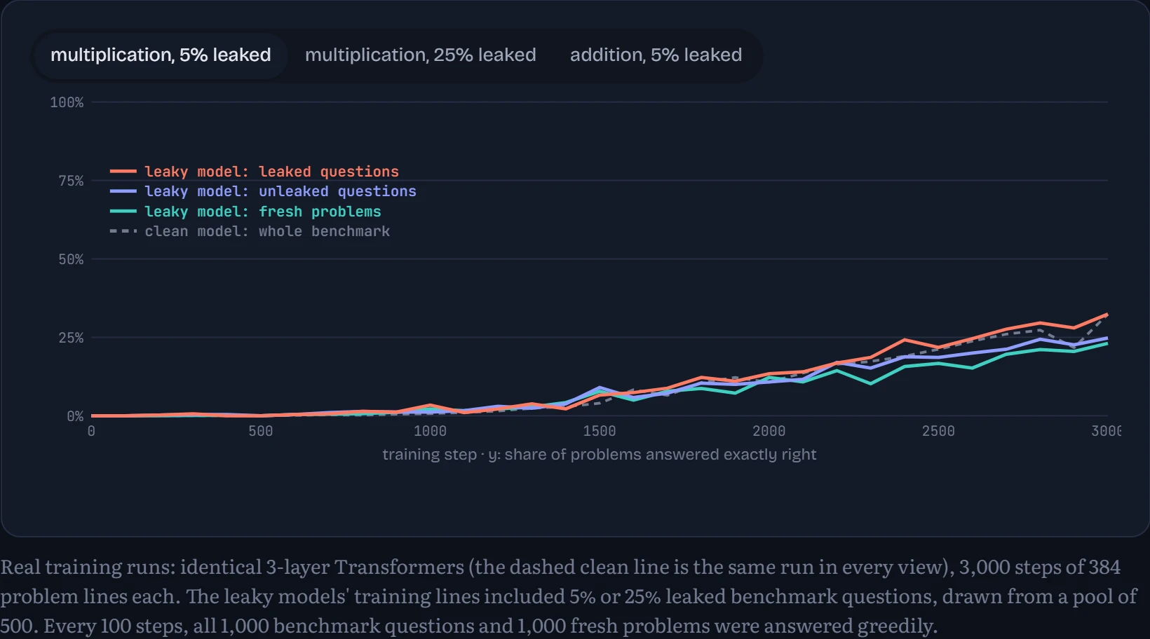
With the heavy leak, the effect is impossible to miss. That model answers 82.4% of the questions it had seen, but only 38.2% of the ones it hadn't, a gap of 44 points created purely by memorization. Averaged over the whole benchmark, it reports 60.3%. The clean model reports 32.4%. A leaderboard would rank the contaminated model 28 points ahead. On fresh problems, the gap is 4 points (36.5% against 32.1%), well within the run-to-run noise. Almost all of the lead is memorization.
The light leak shows the same thing more quietly: leaked questions 32.4%, unleaked 24.8%, a 7.6-point gap inside the same model. Notice that this model's overall score (28.6%) still ended below the clean model's (32.4%): with two separately trained models, the run-to-run variation was as big as the contamination effect. That's why the reliable test compares leaked and unleaked questions within one model, and why the next section is about noise.
Then switch to addition, which surprised me. Same 5% leak, and the leaked and unleaked lines lie on top of each other the whole way (85.0% against 87.2% at the end). The model learned the actual algorithm for addition, and once you can add, a memorized answer is worth nothing extra. Contamination inflates scores most where the model can't really do the task yet, which is exactly where a benchmark is supposed to tell you something. That's why it's so damaging on hard reasoning and knowledge tests. Researchers have measured it in the wild: when Scale AI wrote GSM1k, a fresh look-alike of the GSM8K maths benchmark, some models scored up to about 13 points lower on it than on the original (Zhang and colleagues, 2024).
Labs fight contamination by keeping private test sets, by searching training data for long exact overlaps with benchmark questions, and by planting canary strings, unique random markers in benchmark files, so a model that can complete the canary has clearly seen the file.
Is 2% better really better?
Even with a clean benchmark, a score is a measurement, and measurements are noisy. If a model gets 83% on 100 questions, its “true” accuracy could plausibly be anywhere from about 75% to 90%: a different 100 questions of the same kind would give a different number. Leaderboards routinely rank models separated by less than that noise.
The simplest way to see the noise is the bootstrap: pretend your benchmark is the world, draw a new benchmark of the same size from it at random (with repeats allowed), recompute the score, and do that thousands of times. The spread of those scores tells you how much your number would wobble with a different sample of questions. Below I compare two real checkpoints of the clean multiplication model, 300 training steps apart, on the same questions. In the figure: the benchmark shrunk to a random subset of the real 1,000 questions (the same subset for both models): the smaller it is, the larger the uncertainty.
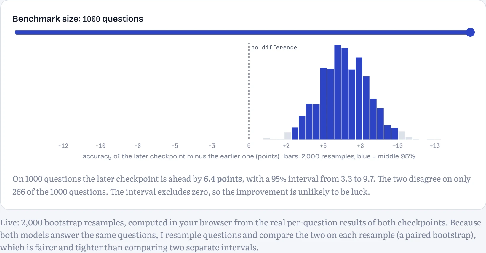
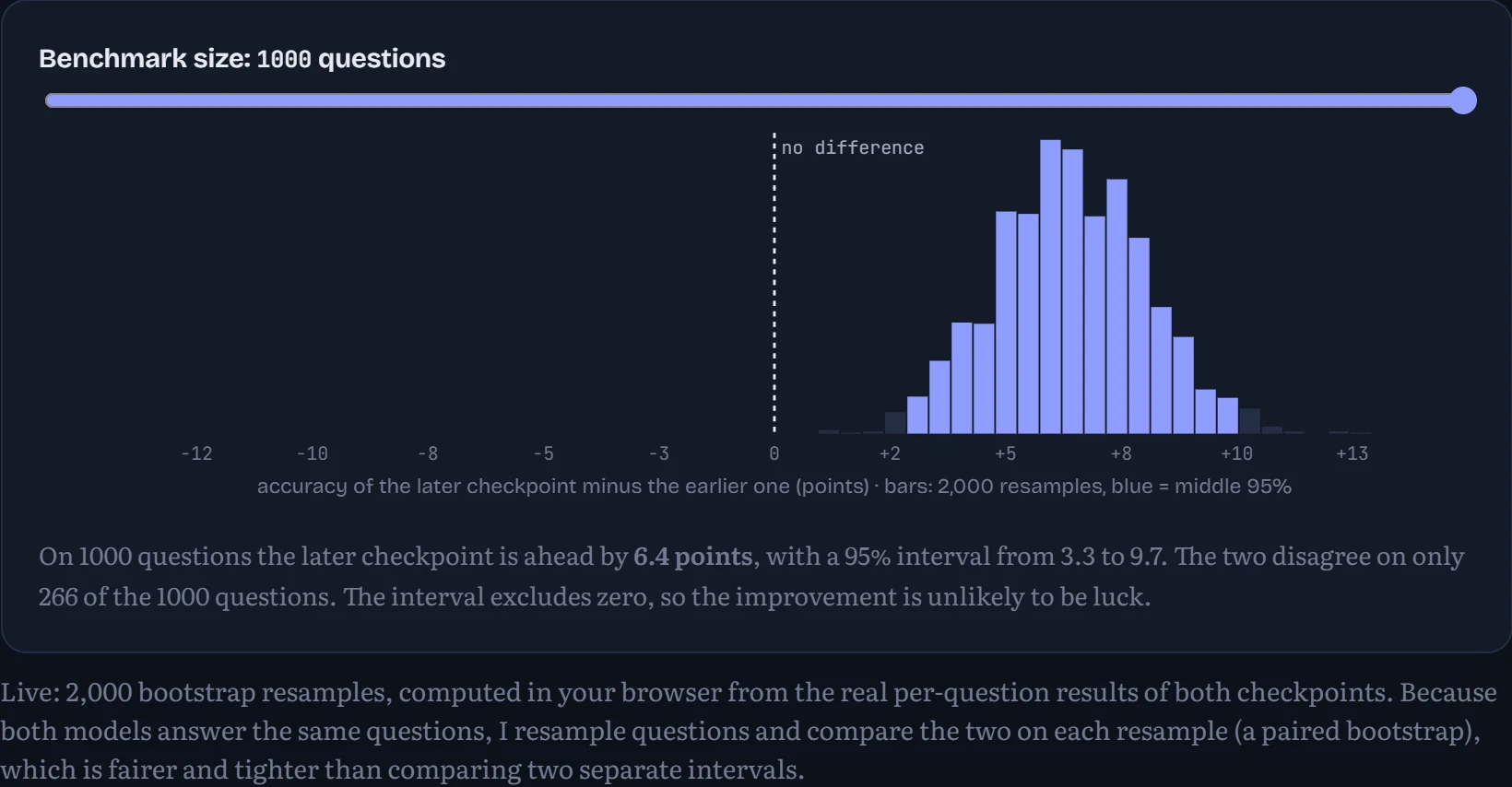
Two habits follow. First, always report an interval, not just a number. Second, when comparing two models, compare them on the same questions and look at where they disagree; most questions are answered the same way by both, and only the disagreements carry information.
Other ways to grade
Addition has one right answer. Most of what we want from language models doesn't: a good summary, a helpful explanation, a safe refusal. Three approaches fill the gap. Human evaluation is the gold standard and the most expensive: people compare two answers side by side, which is also how preference data for RLHF is collected (Chapter 11), and how the public Chatbot Arena ranks models. LLM-as-judge asks a strong model to grade answers. It's cheap and correlates reasonably with people, but has measured biases: judges tend to prefer the first answer shown, longer answers, and answers written in their own style. Swapping the order and averaging, and checking a sample against humans, are standard precautions. Agent evaluations grade outcomes rather than text: did the agent fix the bug so the tests pass, did it book the right flight? Those are closer to what we care about, but slow, expensive and noisy, because an agent takes many steps and can fail at any of them. Whatever you use, the lesson of the bootstrap applies twice over.
Reading the model as it thinks: the logit lens
Benchmarks treat a model as a black box. Interpretability opens the box. The simplest tool is almost cheeky. Remember the residual stream from Chapter 9: one vector per position, which every block reads from and adds to. At the very end, the model turns that vector into a prediction with its final LayerNorm and unembedding. So why not apply that same final step early, after block 1 or block 2, and ask: if the model had to answer right now, what would it say? That's the logit lens (nostalgebraist, 2020).
Here it is on the story model from Chapter 11 (4 blocks, char level), running live. How to read it: each column is one position in your text, and each row is the model's best guess for the next character after reading up to that position, read off after the embeddings (row 0) and after each block. Shading shows how confident that guess is. The top row is the real output; green marks a guess that matches the character that actually comes next.
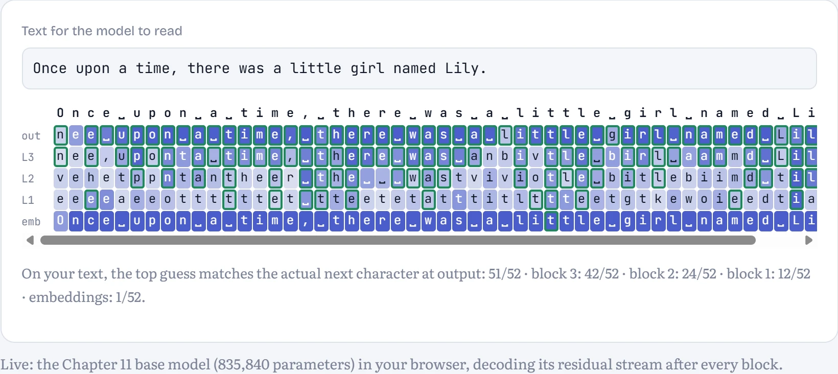
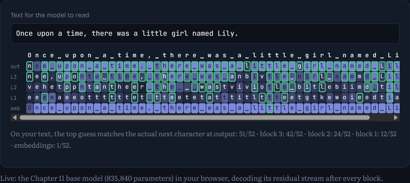
Watch your text's columns from bottom to top. Right after the embeddings, the “prediction” is mostly nonsense: the vector is just the current character plus its position, and decoding it mostly echoes characters back. Each block then adds a little. Measured over 8,192 held-out characters, the top guess was right 2% of the time after the embeddings, 20% of the time after block 1, 34% of the time after block 2, 52% of the time after block 3, 71% of the time after block 4. The model's final answer isn't computed in one place; it's assembled gradually in the residual stream, each block nudging the guess. Easy predictions (the “e” after “th”, a space after a full stop) often settle early; anything that needs context, like the rest of a name mentioned earlier, settles late. That gradual refinement is exactly what the residual-stream picture from Chapter 9 promised, and the logit lens lets you see it. (It works less cleanly on big models, whose early layers use a different “language” from the output; a variant called the tuned lens learns a small translation per layer.)
Probing: is that information in there?
The logit lens asks what the model would predict. A probe asks what it knows. Pick a property you suspect the model tracks, collect its internal vectors at many positions, and train a tiny classifier (here, a linear one: a single weighted sum) to read the property off those vectors. If a simple probe succeeds, the information is sitting there in an easily readable form.
I picked something a story model must track to write dialogue properly: is the current character inside a quotation? To close a quote at the right moment, the model has to remember whether one is open, which depends on how many quote marks came before, possibly a hundred characters back. How to read the chart: each pair of bars is one layer of the model. The blue bar is how often a linear probe on that layer's vectors correctly says “inside a quote” or “not”, on positions it wasn't trained on. The dashed line is the score you'd get by always guessing the more common answer, so only the height above it counts. The grey bar is a control task, explained below.
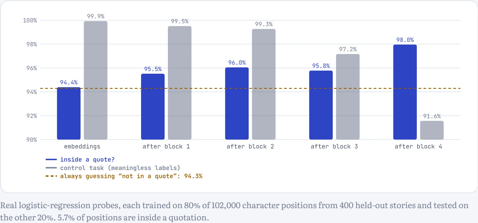
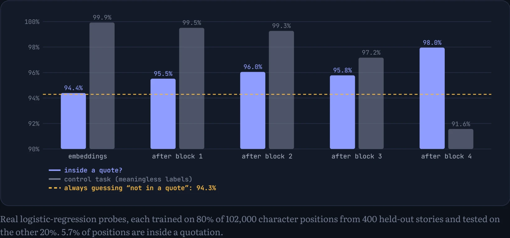
Only 5.7% of characters are inside a quotation, so “always no” already scores 94.3%; what matters is how many of the remaining mistakes the probe removes. On the raw embeddings, almost none: 5.6% error. After the last block, 2.0%, so the probe gets roughly 64% of the baseline's mistakes right, with the biggest single improvement coming in block 4. Before any block has run, the probe is near baseline; the information appears as the blocks look back across the text, which only attention can do.
Now the grey bars, which are the cautionary tale. The control task gives every character type a random label, such as “every ‘k’ is class 1, every ‘m’ is class 0”: a property with no meaning that the model has no reason to track. The probe still gets 99.9% on the embeddings, because a linear probe can read character identity off the embedding and memorize the random table. A probe can find anything that's decodable, whether or not the model uses it. The control score falls in later layers (91.6% at the end) as the vector fills with information about the next character instead of the current one, while the quote score rises. That contrast is what makes the quote result convincing. The firmer test is causal: change the direction the probe found and see whether the model starts closing quotes at the wrong time. The next section does that kind of experiment on a circuit.
A circuit, found and verified
Probes show that information exists. The deeper goal, called mechanistic interpretability, is to find the actual algorithm: which components do what, and how they connect. The best-understood example is the induction head (Olsson and colleagues at Anthropic, 2022). It implements a rule you use constantly when reading: if this token appeared before, predict whatever came after it last time. Having read “Mr Dursley … Mr”, you expect “Dursley”.
It takes two attention heads working together, in different layers. A previous-token head in an early layer copies each position's previous token into its vector, so the vector for “Dursley” now also says “I come right after Mr”. Then the induction head, in a later layer, sitting at the latest “Mr”, searches for positions whose vector says “I come after Mr”, finds “Dursley”, attends to it, and copies it to the output. Two simple steps, chained, give the model a form of in-context learning.
I went looking for induction heads in our own models, and the first result was a surprise: there weren't any. I fed the Chapter 11 story model a string of random words, then the same string again. A model with induction heads finds the second copy far easier, since it can just copy. Ours found it no easier at all: its loss was 2.08 on the first copy and 2.21 on the second. I then trained a fresh 2-layer attention-only model on stories for 4,000 steps: same story (2.60 versus 2.60). Both models had seen tens of millions of characters. The original paper saw induction heads appear after roughly a few billion tokens of training. Our story models simply hadn't been trained long enough for copying from context to beat the cheaper local patterns they were busy learning.
So I changed the diet, not the model. A fresh copy of the same 51,584-parameter attention-only model (2 layers, 4 heads each, no MLPs) was trained with half of each batch from stories and half from text where copying pays off immediately: a random chunk of 8 to 32 letters, repeated over and over, like qkjznounkwkjxdkhphrseqkjznounkwkjxdkhphrseqkjzno…. The chunk length varies, so the model can't just look a fixed distance back; it has to match content. How to read the chart: the blue line is the loss on the second copy of a repeated random sequence (lower means it's copying), the grey line the loss on the first, uncopyable copy, and the amber line (right axis) the strongest induction-style attention any second-layer head shows.
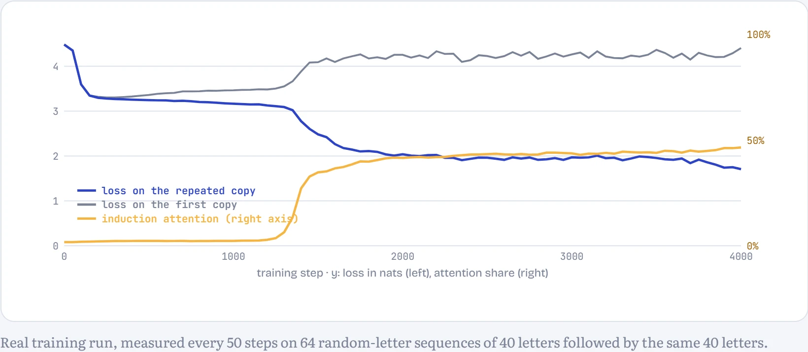
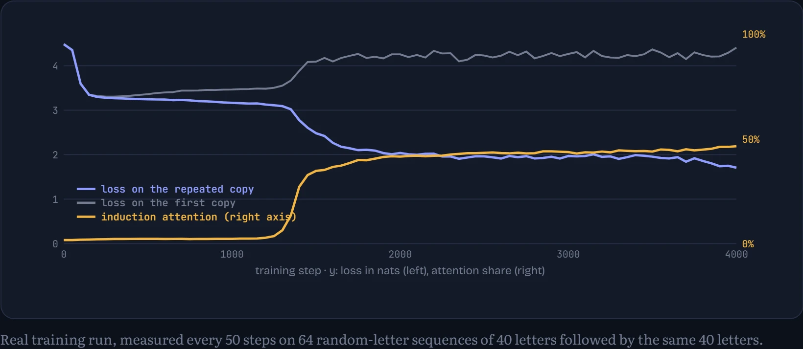
For the first 1,300 steps, nothing happens to copying. The loss on the repeated copy hovers around 3.15 nats, close to ln 26 ≈ 3.26, the cost of guessing uniformly among 26 letters: the model has learned that these stretches are random letters, and nothing more. (The first copy costs even more, 4.4 nats by the end, because the model's English habits make random letters look extra unlikely.) Then, around step 1,350, the strongest induction attention jumps from about 2% to over 30% in a few hundred steps, and the repeated-copy loss plunges with it, below 2.2 nats by step 1,650. It ends at 1.71 nats. A sudden jump after a long plateau is the signature the original paper called a phase change. The circuit needs two heads in different layers to work together, and neither is useful on its own, so training wanders on the plateau until the two click into place.
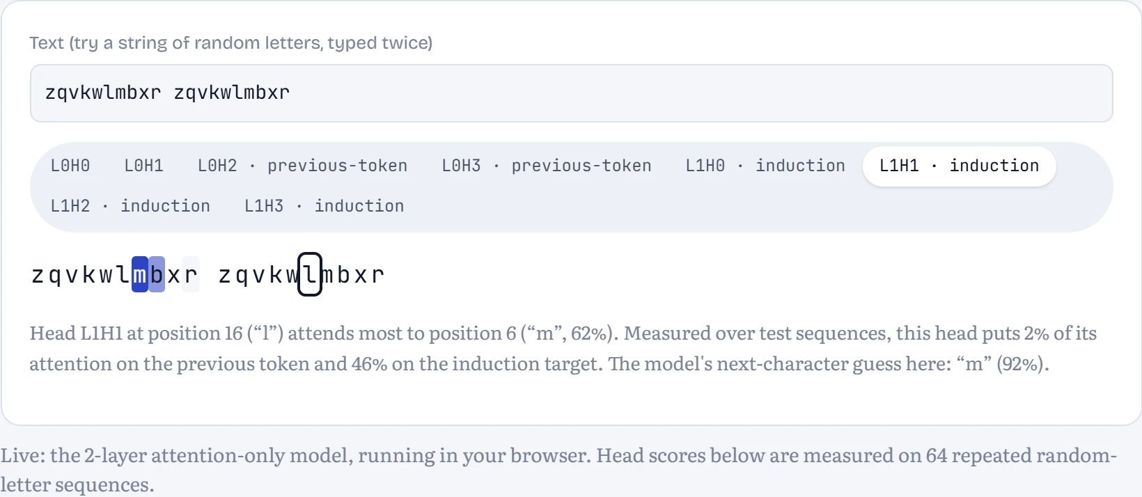
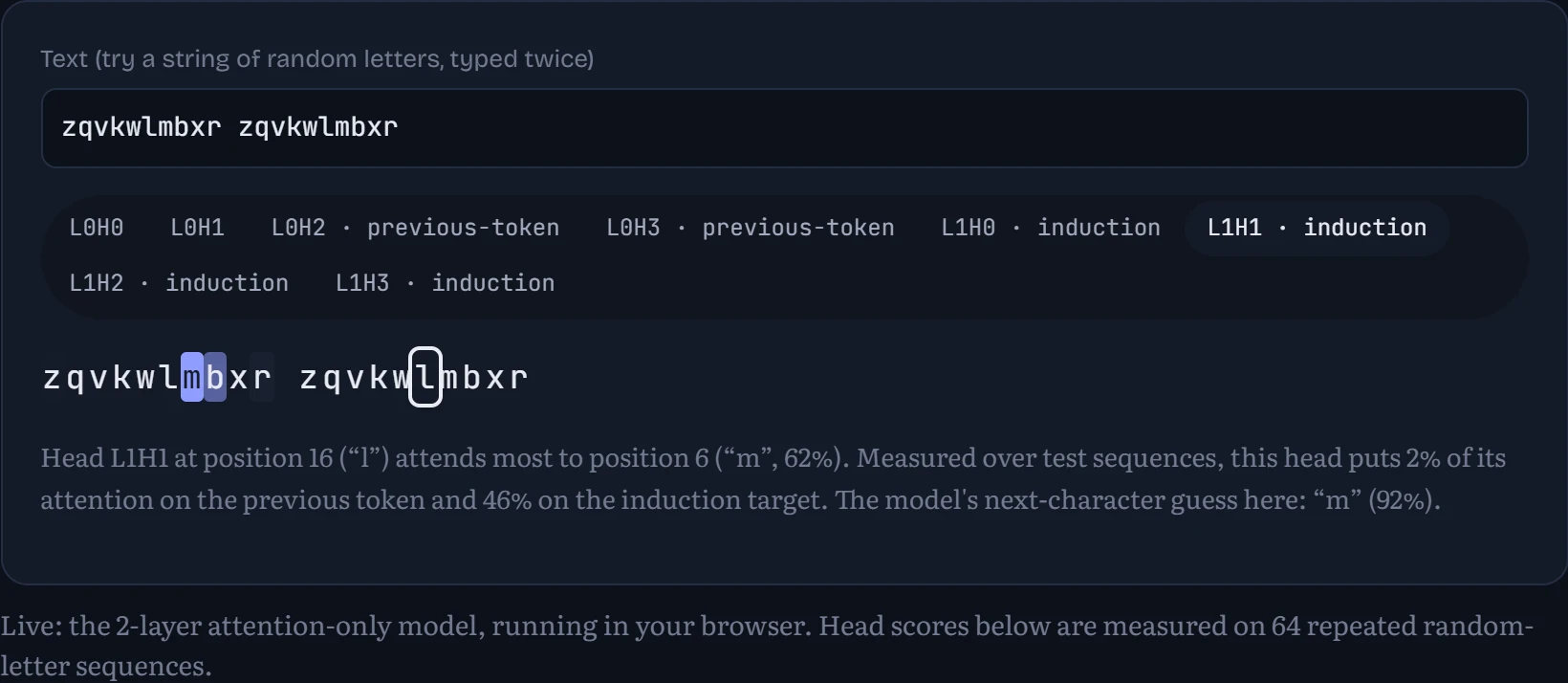
Now let's look at the heads themselves, live. How to read it: the shading shows how much that head, at that position, attends to every earlier character. The previous-token head should light up the character just before; an induction head, sitting in the second copy of a repeated chunk, should light up the character after the matching spot in the first copy. The default text is a nonsense string typed twice, because that's the kind of text this model practised copying on. there, its induction heads are much quieter. The circuit formed where the data rewarded it, and it generalizes only partly beyond that, another reminder that what a model learns is shaped by what it was trained on.
Watching attention is suggestive, not proof. To show a component causes a behaviour, interpretability researchers intervene. Two standard experiments: ablation switches one head off (sets its output to zero) and measures how much worse the model gets at copying. Activation patching is subtler. Run the model on a “corrupted” input where copying is impossible (the first half replaced by different random letters), then paste in one head's output from the clean run and see how much of the copying ability comes back. If pasting one head restores most of it, that head carries the information. How to read the grids: rows are layers, columns are heads.
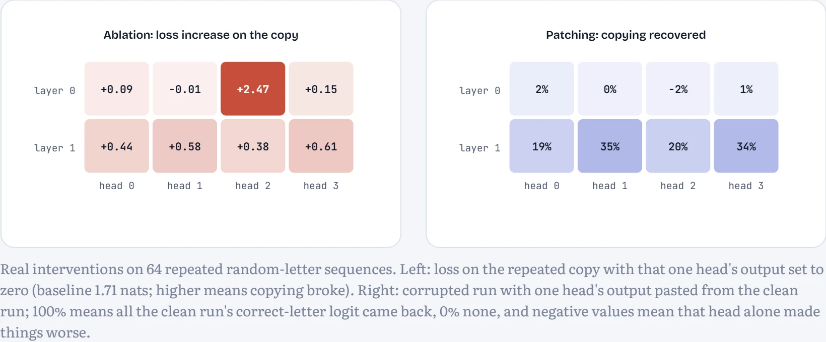
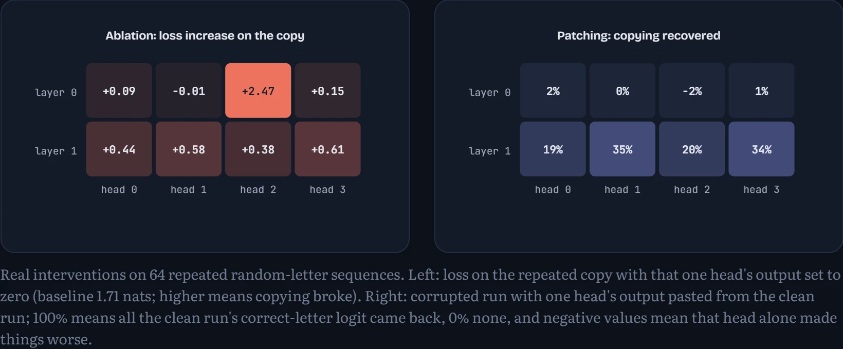
The two experiments tell complementary stories. Ablation singles out L0H2: switching it off pushes the copying loss from 1.71 to 4.17 nats, worse than not copying at all, while every other head costs far less. It's the previous-token head (it puts 58% of its attention on the character just before). Without it, no second-layer head can find the earlier copy, because the “what came before me” information they search for is never written. One head, and the whole circuit fails. The second layer is different: all four heads became induction heads, and ablating any one of them costs only 0.38 to 0.61 nats, because the others keep copying. The work is shared.
Patching agrees from the other direction. Pasting any single second-layer head's clean output into the corrupted run restores 19% to 35% of the copying signal: each carries part of the answer, and none carries all of it. Patching a first-layer head restores almost nothing (at most 2%), and that's informative too. In the corrupted run, the first half contains different letters, so even if a patched previous-token head helps the induction heads find the right position, what they copy from there is the corrupted letter. The previous-token head is essential but not sufficient; it tells the copier where to look, not what to say. This is mechanistic interpretability in miniature: form a hypothesis from attention patterns, then confirm it with interventions whose results would have come out differently if the hypothesis were wrong.
Superposition: more ideas than dimensions
If you look at single neurons in a language model, most are a mess: one neuron might fire for academic citations, Korean text and HTTP requests. Why would a model tangle unrelated concepts together? Anthropic's toy-model work (Elhage and colleagues, 2022) gave a clean answer: because it has more things to represent than it has dimensions, and it can get away with sharing.
You can watch this happen in a model small enough to draw. It has to squeeze 5 input features through a 2-dimensional bottleneck and rebuild them on the other side (output = ReLU(Wᵀ·W·x + b)). Each feature gets a direction in the 2-D space, drawn below as an arrow. Feature 1 matters most to the loss, feature 5 least. The key knob is sparsity: how often each feature is zero. Real-world features are very sparse; any given sentence mentions almost none of the concepts a model knows. In the figure: the model after training at one sparsity.
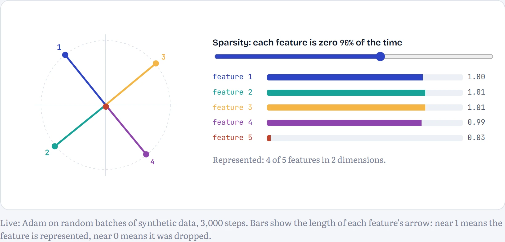
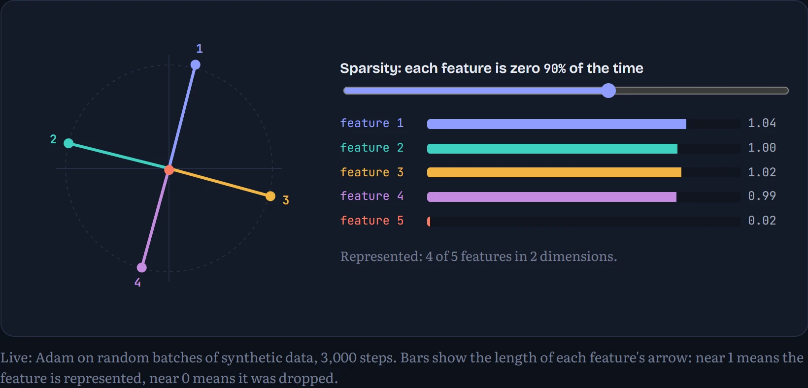
With dense features (sparsity 0%), the model does the obvious thing: it gives its two dimensions to the two most important features and ignores the rest. As features get sparser, it starts packing in more, as arrows at angles to each other. That causes interference (when two features are active at once, they bleed into each other), but if they're rarely active together, the occasional error costs less than dropping a feature entirely. The ReLU and the bias clean up small leaks. That trade-off is superposition, and it's why individual neurons in real models are hard to read: concepts are stored as directions that don't line up with neurons, many more directions than neurons.
Sparse autoencoders: untangling the features
If concepts are directions in superposition, can we find the directions? A sparse autoencoder (SAE) tries. It's a second, separate network trained to rebuild the model's internal vectors through a much wider layer, with a penalty that keeps almost all of that layer at zero at any moment. Each unit of the wide layer is a candidate “feature”, and the sparsity pressure pushes each one towards meaning one thing. Anthropic's “Towards Monosemanticity” (2023) and “Scaling Monosemanticity” (2024) used this approach to find millions of interpretable features in production models, including the famous Golden Gate Bridge feature which, when turned up, made Claude bring up the bridge in every answer.
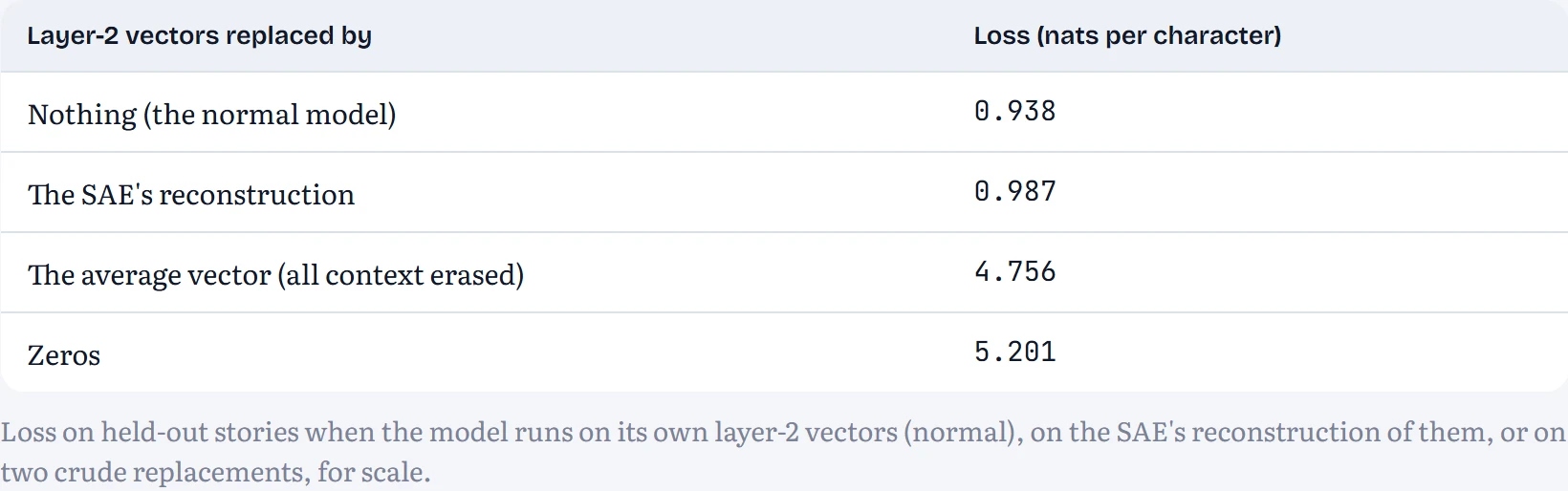
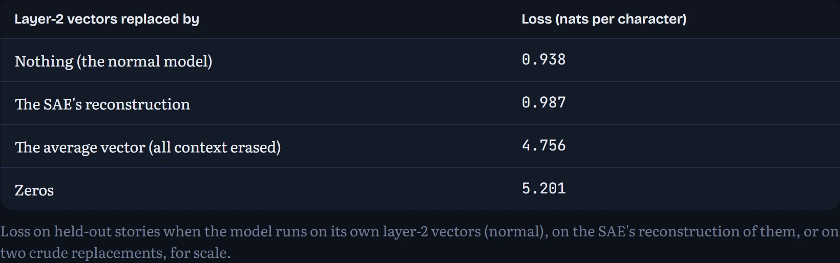
I trained one on the Chapter 11 story model's residual stream after block 2: 128 numbers per position, expanded to 1,024 candidate features. After training, about 62 features are active on a typical character (out of 1,024), 0.0% of features never fire on held-out text, and the reconstruction misses 3.1% of the variance in the vectors. Is that good enough? The real test is to run the rest of the model on the SAE's reconstruction instead of the real vectors and see how much worse its predictions get.
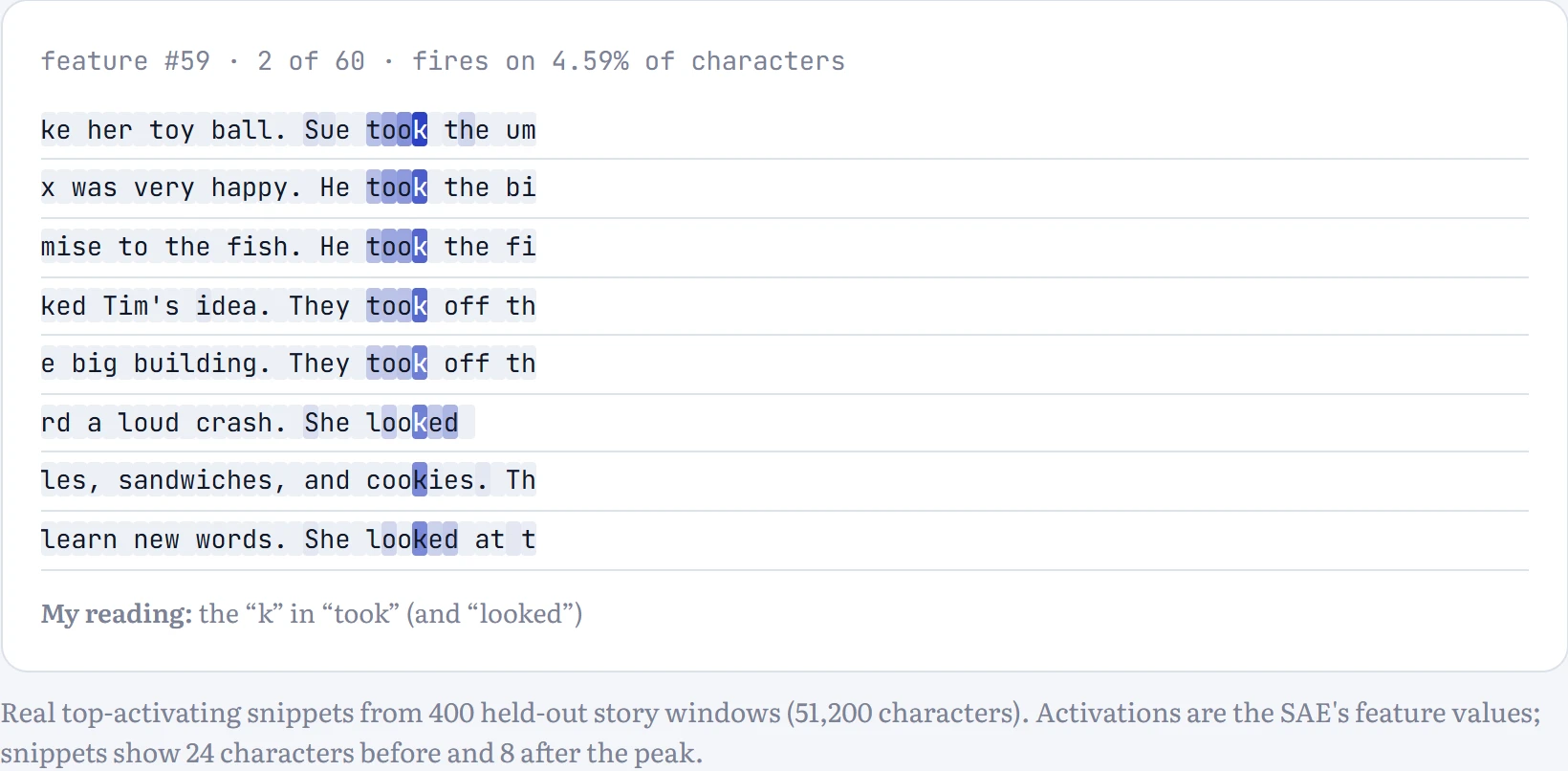
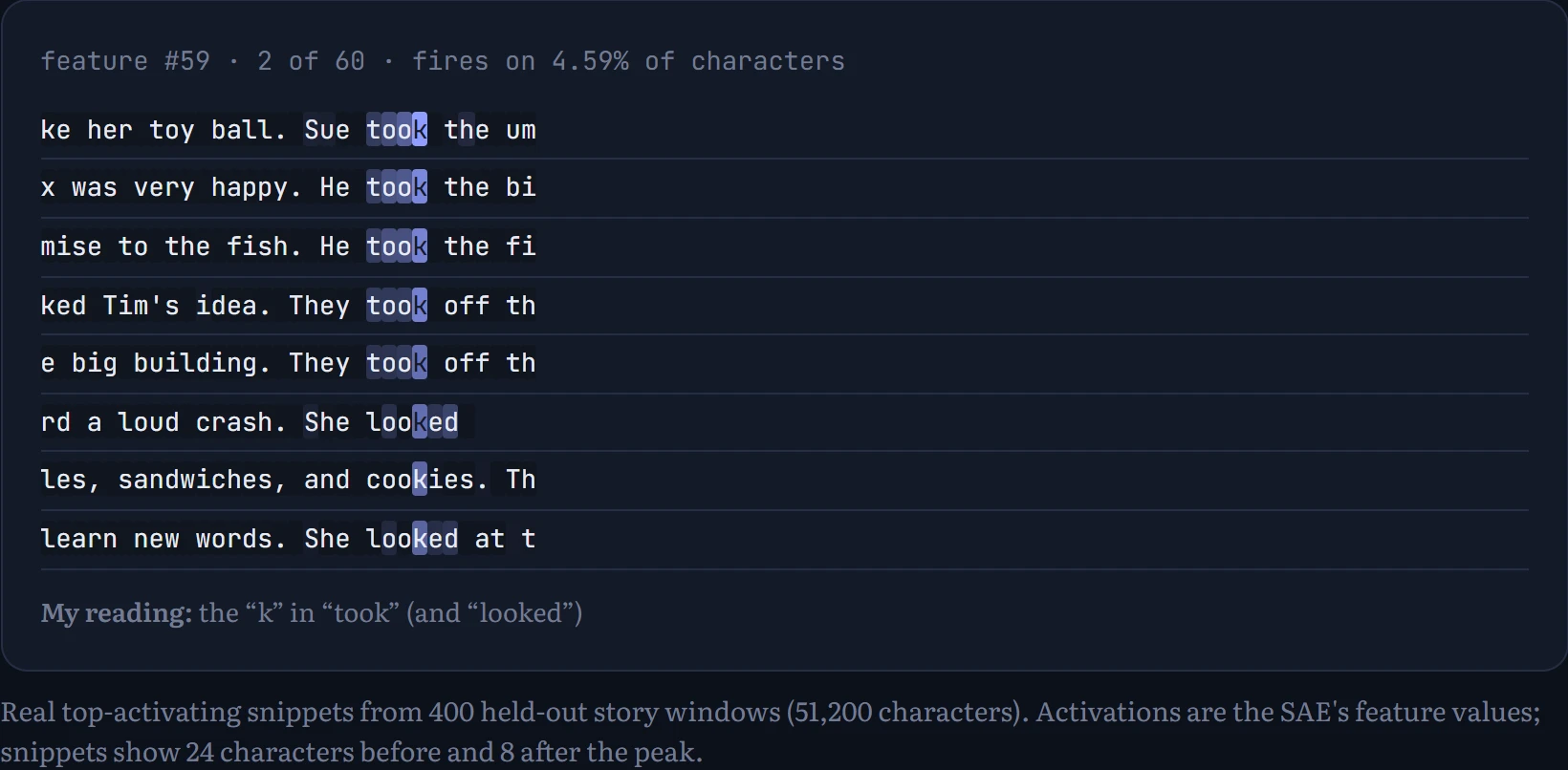
Now the fun part: what did the features learn? Below is a browser of 60 features chosen at random (from those that fire on between 0.1% and 10% of characters; I didn't cherry-pick). How to read it: each line is one of the text snippets that made this feature fire most strongly, and darker highlighting means stronger activation on that character. Read a few lines and guess what the feature means before looking at my reading.
On the table: erasing all context from the layer-2 vectors (replacing them with their average) pushes the loss from 0.94 to 4.76. Running on the SAE's reconstruction gives 0.99, so the SAE preserves about 99% of what those vectors contribute, while describing each character with roughly 62 active features instead of 128 tangled numbers. As for meaning: of the 60 random features in the browser, I could give a confident one-line description to 44 after reading their top examples; the rest looked like mixtures, or patterns I couldn't name. That ratio is typical of small SAEs, and it's an honest picture of the tool: real structure, partly legible.
Notice what kind of features they are. Almost all of them are about spelling: “I'm inside the word took, the next letter is k”, “this is the u in would”, “this is the i in the name Lily”. A few track structure instead: the start of a new paragraph, a question mark closing a question, the full stop that ends a sentence introducing a character. That's a fair portrait of what a small character-level model is busy with halfway through its stack: recognizing words from their letters, and keeping track of where it is in a sentence. In large models, SAEs find features at a much higher level, such as particular people, places, emotions, code bugs or deception, because that's what those models need to represent.
OPEN RESEARCH. SAEs are a young tool with open problems. Features can split or merge depending on the dictionary size, a fraction are uninterpretable, the reconstruction always loses something (the “dark matter” the SAE fails to explain), and a feature that looks clean on its top examples may fire on unrelated things at weaker strengths. Newer variants (transcoders, crosscoders, attribution graphs that trace features across layers) aim to explain computation, not just representation. Whether this scales to a complete understanding of a frontier model is one of the field's big open questions.
Continue the lesson
The whole lesson, with its drawings and its questions. 7 more sections after the ones above.