
Post-training: SFT, LoRA and QLoRA, distillation, RLHF, DPO and KL-regularised RL
A base model only continues text in the style of its training data. Post-training turns it into something you can talk to, in two broad steps: supervised fine-tuning on examples of the behaviour you want, then learning from feedback on its own outputs, such as which answer was better or whether it was right.
What this page answers
What is supervised fine-tuning?
Training a base model further on examples of exactly the behaviour you want, a request followed by a good response, with the same next-token loss used in pre-training. Only the data changes. Read it in “Teaching by example: supervised fine-tuning”
What is the difference between RLHF and DPO?
Both learn from preferences between two answers. RLHF trains a reward model on the preferences and then optimises against it with reinforcement learning; DPO turns the preferences directly into a loss on the model. Read it in the lesson
What a base model is, and isn't
Our base model is the same kind of small Transformer you built in Chapter 9: 836K parameters, a 256-character context window, trained for 3,000 steps on 21 million characters of TinyStories (Chapter 10), short children's stories. Its held-out loss ended at 0.96 nats per character.
A base model has exactly one skill: given some text, predict what comes next, in the style of its training data. It has no notion of “a request” or “an answer”. If you type a question, it may answer it, or continue with three more questions, or start a new story, depending on what usually followed text like yours in its training data. Our base model read twenty million characters of children's stories and has never once seen the words “Write a story about”. So when it sees them, it does what it always does: it continues, and the instruction is just more text to continue.
Everything that turns a model like this into something you can talk to is called post-training. It usually happens in two broad steps. First, show it examples of the behaviour you want (supervised fine-tuning). Then, push it further using judgements of its own outputs: which answer was better, or simply whether it was right (learning from feedback).
Teaching by example: supervised fine-tuning
The first step is almost disappointingly simple. Collect examples of exactly the behaviour you want, a request followed by a good response, and keep training the base model on them with the same next-token loss you already know. Nothing about the network changes. Only the data changes, and the model's habits follow the data.
One detail matters: you only train on the response. The request is fed in so the model can read it, but its tokens are left out of the loss, because the goal is to learn how to answer, not how to ask. Real assistants also wrap every turn in a fixed chat template, with special tokens marking who is speaking, so the model always knows where your message ends and its reply should begin. Here's what one training example looks like, with the trained part highlighted:
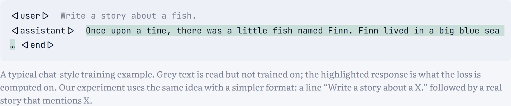
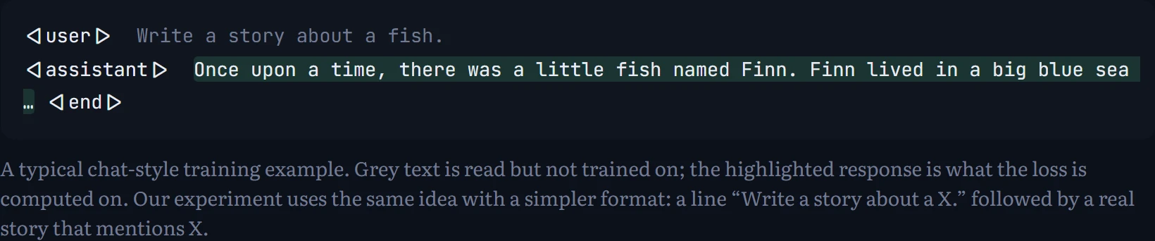
For our experiment I built 9,057 training examples automatically: for each training story that mentions one of twelve simple topics (dog, cat, ball, bird, fish, tree, car, boat, cake, flower, bear, frog), the prompt is “Write a story about a <topic>.” and the response is the story itself. Each chosen story mentions its topic within its first 120 characters, the way a good answer gets to the point. Then I fine-tuned the base model on them for 1500 steps, which took 4 minutes.
So did it work? The chart below counts, for each of twelve topics, how often the model's story actually mentions the requested thing. How to read it: each group of three bars is one topic. The grey bar is the untouched base model, the blue bar is after full fine-tuning, and the teal bar is after LoRA fine-tuning (explained in the next section). Taller means the model followed the instruction more often; a perfect instruction-follower would reach the top every time.
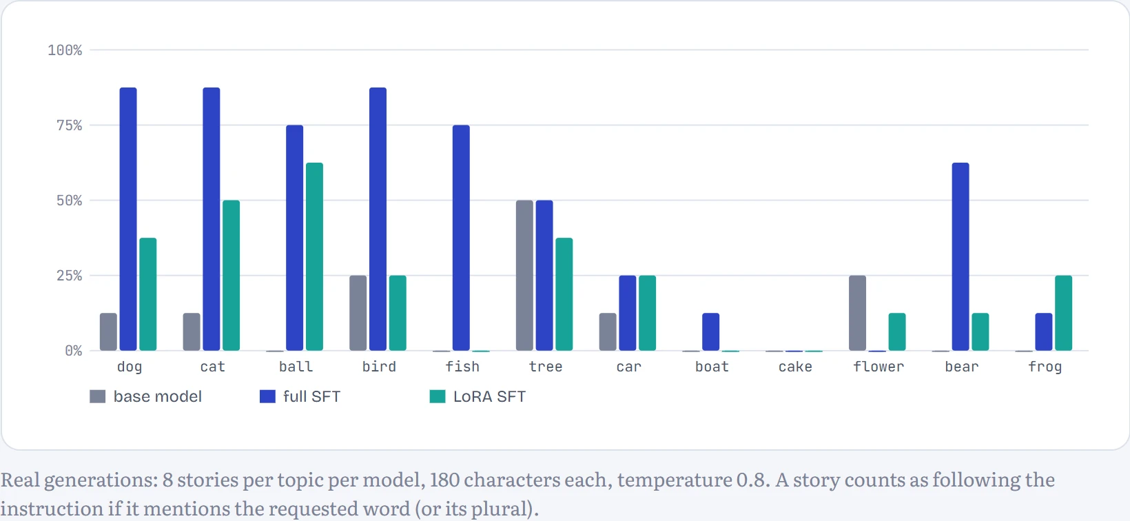
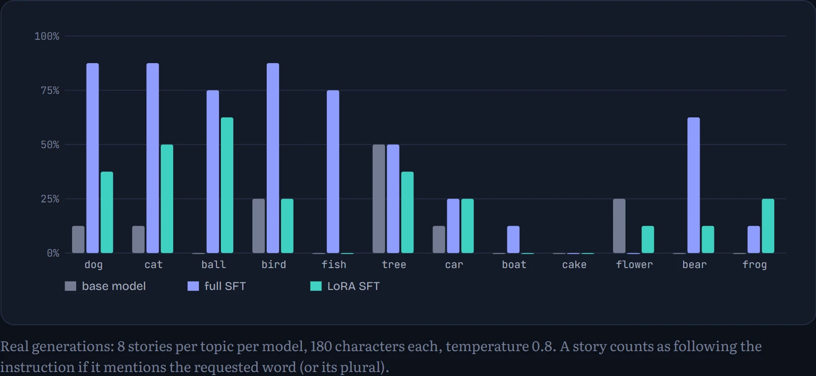
Averaged over all twelve topics, the base model's stories mention the requested thing 11% of the time. That's not zero, because children's stories mention dogs and balls anyway; it's roughly the rate you'd get by ignoring the instruction completely. After fine-tuning, it's 48%. The model has learned that the first line is a request, and that the story should be about it. It isn't perfect, and it isn't free: its loss on ordinary held-out stories rose a little, from 0.956 to 1.072, because it now spends some of its effort on the new format. That small loss of general skill is a mild case of what's called catastrophic forgetting, and keeping it small is why fine-tuning runs are short and use low learning rates.
A note on data. Real instruction datasets are written or checked by people, or generated by other models and filtered, and they're tiny compared with pre-training data: tens of thousands to a few million examples rather than trillions of tokens. Quality matters far more than quantity here, a finding sometimes summarized as “a little high-quality data goes a long way”. The flip side is that the model copies whatever habits the examples have, good or bad, including their length, tone and mistakes.
LoRA: changing a model by adjusting a tiny add-on
Full fine-tuning updates every weight, which for a large model means holding all the gradients and optimizer states in memory (16 bytes per parameter, Chapter 10) and saving a complete new copy of the model for every task. LoRA, short for low-rank adaptation, avoids nearly all of that.
The idea: freeze the original weight matrix W and learn a small correction alongside it. The correction is written as the product of two thin matrices, B (tall and narrow) and A (short and wide), so the layer computes W·x + (α/r)·B·A·x. If W is 4,096 × 4,096, that's about 16.8 million numbers; with a rank r of 16, B and A together hold only about 131 thousand. Think of it as writing corrections on a few sticky notes instead of reprinting the whole book. B starts at zero, so at the beginning the add-on does nothing and the model behaves exactly like the original.
Why would such a thin correction be enough? Because adapting a model to a new task seems to need only a few new “directions” of change, not a complete rewrite. That's an empirical finding from the LoRA paper (Hu and colleagues, 2021), on large models. On our tiny one it was only partly true, as you'll see below.
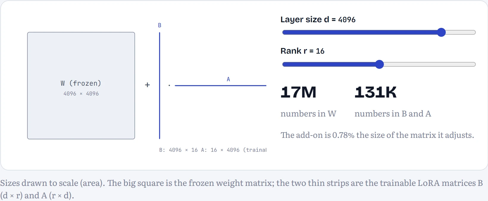
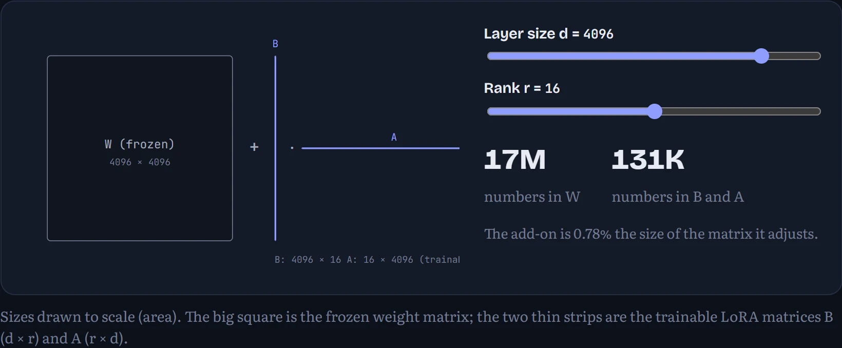
In our experiment, LoRA with rank 8 on every attention and MLP matrix trained 65,536 numbers instead of all 835,840, about 8% of the model. (On a model this small the add-ons are a big share; on a 7-billion-parameter model, rank 16 is typically well under 1%.) It reached 24% instruction-following, against 48% for full fine-tuning and 11% before either, with the same number of steps. So here LoRA captured only part of the improvement. A model this small has little spare capacity for a rank-8 add-on to steer, and our learning rate wasn't tuned for it; on large models the gap between LoRA and full fine-tuning is usually much smaller. Since only B and A change, you can keep one copy of the base model and swap in a small file per task, or merge B·A into W afterwards so there's no extra cost at all when the model runs. A popular variant, QLoRA, also stores the frozen W in 4 bits, which is how people fine-tune multi-billion-parameter models on a single consumer GPU.
QLoRA: fine-tuning a model that's been squeezed to 4 bits
LoRA shrinks what you train, but the frozen base model still has to sit in memory. QLoRA (Dettmers and colleagues, 2023) shrinks that too: store the frozen weights in 4 bits instead of 16 or 32, and train the LoRA add-on on top in full precision. Four bits means only 16 possible values per weight. The trick is choosing them well. Trained weights are roughly bell-shaped, mostly near zero, so NF4 (“normal float 4”) places its 16 levels where a bell curve puts its values, close together near zero and sparse at the edges, and stores one scale number for every block of 64 weights. That's how a 65-billion-parameter model became fine-tunable on a single 48 GB GPU.
How much does 4 bits cost? How to read the chart: the base model's loss on held-out stories with its attention and MLP weights rounded to each format (lower is better).
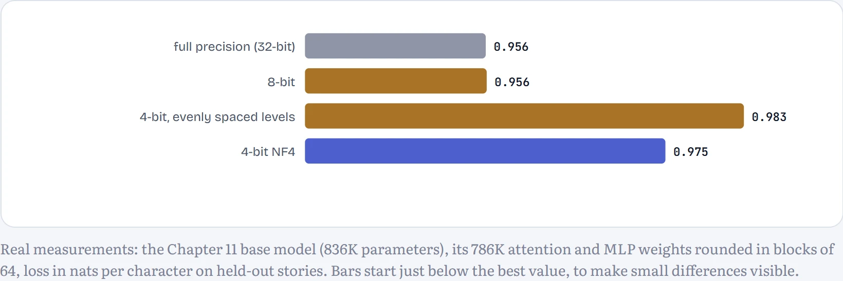
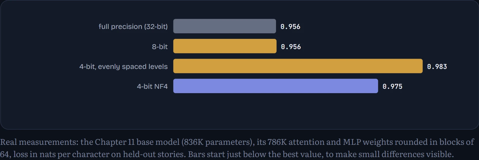
Eight bits is free: 0.956 against 0.956. Four bits costs something, and how you spend the 16 levels matters: evenly spaced levels lose 0.027 nats, NF4's bell-shaped levels only 0.019, 30% less damage for the same 4 bits. The LoRA add-on trained on top can then learn to compensate for some of what rounding lost.
Four ways to adapt the same model
LoRA isn't the only parameter-efficient method. The older one is adapters (Houlsby and colleagues, 2019): insert small bottleneck layers after the attention and MLP blocks, which squeeze the signal down to a few numbers and back up, and train only those. Unlike LoRA, an adapter can't be folded back into the original weights afterwards, so it adds a little computation to every prediction forever. I fine-tuned the Chapter 11 base model on the same “Write a story about a X” task four ways, all for 800 steps. How to read the table: how many numbers each method trained, how much memory the model's weights need, the loss on held-out instruction examples (lower is better) and how often the stories actually mention the requested topic.
| Method | Numbers trained | Memory for the weights | Held-out task loss | Stories on topic |
|---|---|---|---|---|
| no fine-tuning (base model) | – | 3.34 MB | 0.777 | 11% |
| full fine-tuning | 835,840 (100.0%) | 3.34 MB | 0.652 | 33% |
| LoRA (rank 8) | 65,536 (7.8%) | 3.34 MB | 0.688 | 17% |
| QLoRA (rank 8, 4-bit base) | 65,536 (7.8%) | 601 KB | 0.690 | 16% |
| adapters (bottleneck 16) | 33,920 (4.1%) | 3.34 MB | 0.709 | 26% |
Every method improved on the base model (task loss 0.777, on topic 11%). Full fine-tuning, which changes all 835,840 numbers, did best (0.652, on topic 33%). LoRA trained 8% as many numbers and reached 0.688; QLoRA, with the frozen weights squeezed to 4 bits, reached 0.690 while needing 601 KB for the weights instead of 3.34 MB. That's essentially no penalty for the 4-bit base, which is the QLoRA paper's main finding, reproduced at tiny scale. Adapters reached 0.709 with 33,920 trained numbers.
The topic-following column is noisier (96 sampled stories per method), and on a model this small the parameter-efficient methods recover only part of what full fine-tuning gains, the same caveat as the LoRA result above. At real scale the ranking usually tightens: on billion-parameter models LoRA and QLoRA typically come within a few points of full fine-tuning, which is why nearly everyone fine-tuning an open model on one GPU uses them. The memory column is the decisive one there: a 7-billion-parameter model needs about 14 GB in 16-bit just to load, and about 4 GB in 4-bit.
Distillation: a small model learning from a big one
The third way to get a cheap, capable model is to train a small one to imitate a large one. Ordinary training gives the student only the right answer for each position (“the next character is e”). Distillation (Hinton and colleagues, 2015) also gives it the teacher's whole probability distribution: “e is likely, a is plausible, z is absurd”. Those near-misses carry information the hard label throws away, often called the teacher's dark knowledge. Many small models you can download today were made this way from larger ones. I trained a student with a quarter of the base model's parameters twice from scratch on the same data: once on plain labels, once on half labels, half the teacher's softened probabilities. How to read the chart: held-out loss during training; the dotted line is the teacher.
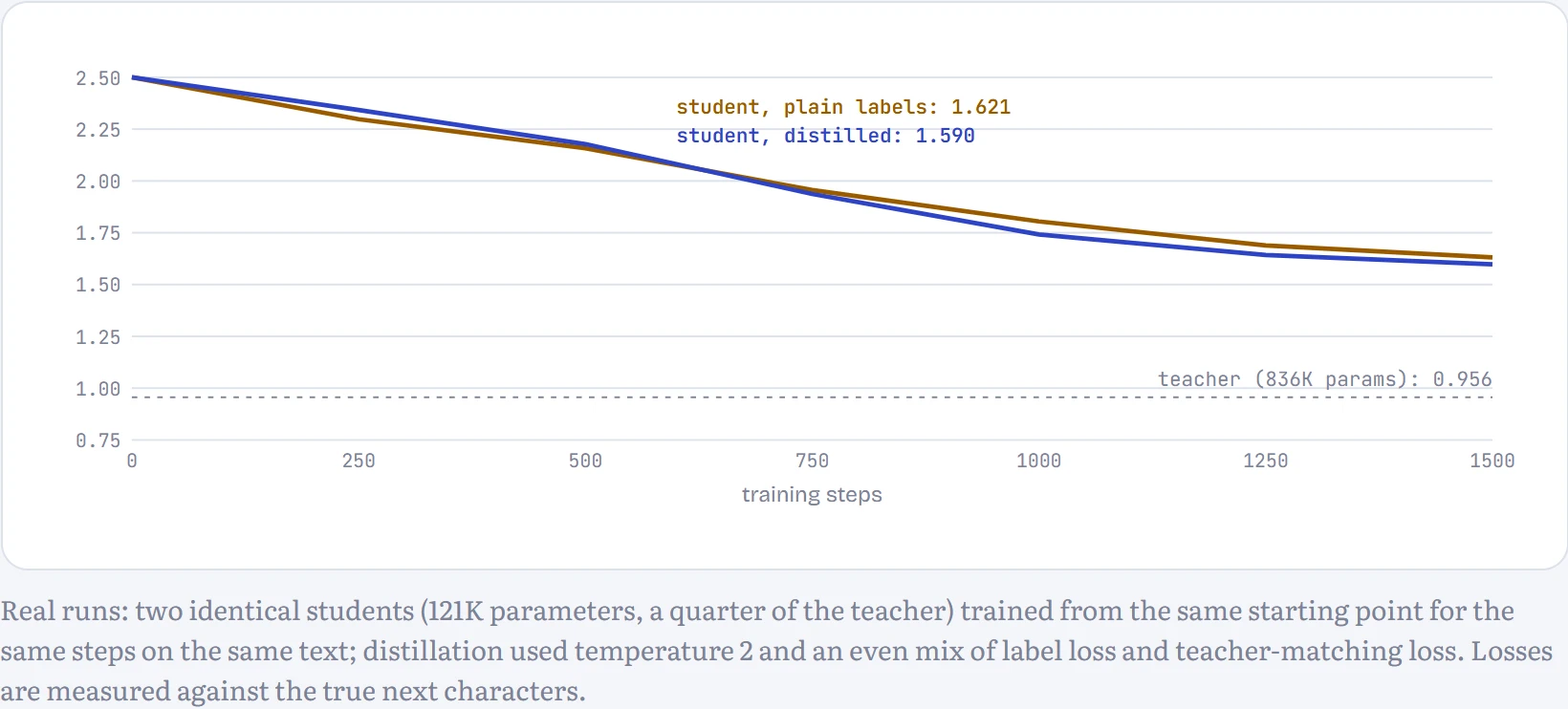
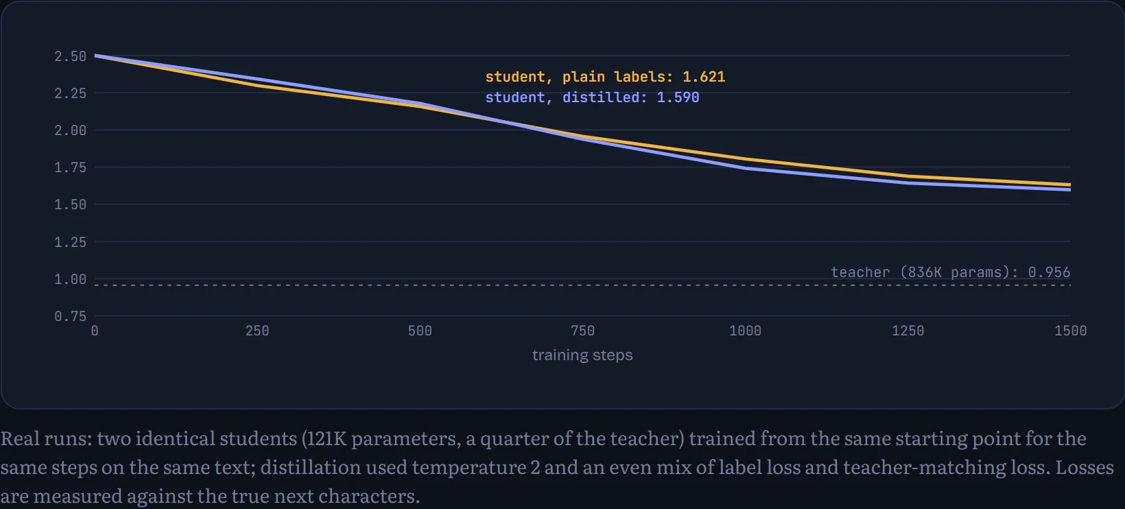
The distilled student ended at 1.590 against 1.621 for the one trained on labels alone: better at predicting the real text, although half its training signal came from imitating another model rather than from the text itself. Neither gets near the teacher: a model a quarter the size can't hold everything the larger one knows, and distillation is a way to lose less, not to lose nothing. The advantage comes from the soft targets: at each position the student learns how plausible every alternative character is, not just which one happened.
Learning from rewards: the core idea of RL
Supervised fine-tuning needs someone to write the perfect answer. Often you can't: what's the single perfect poem, or the best way to explain a concept? But you can often judge answers, or check them. Reinforcement learning works from judgements alone.
Here's the whole idea in one sentence: let the model try things, then make the tries that went well more likely and the tries that went badly less likely. In RL vocabulary, the model is a policy (it chooses actions; for a language model, each next token is an action), the judgement is a reward, and the update rule that does exactly what that sentence says is called REINFORCE: nudge up the log-probability of each sampled action in proportion to how good its result was.
There's one important refinement. If every reward is positive, every try gets made more likely, just some more than others, and learning is slow and noisy. Instead, compare each result with what you'd normally expect, a baseline, and use the difference, called the advantage. Better than usual: push it up. Worse than usual: push it down. The cleanest way to see this is with a toy. Below are five slot machines with hidden payout rates. The “policy” is just five probabilities for which machine to play; it learns from nothing but the payouts it receives.
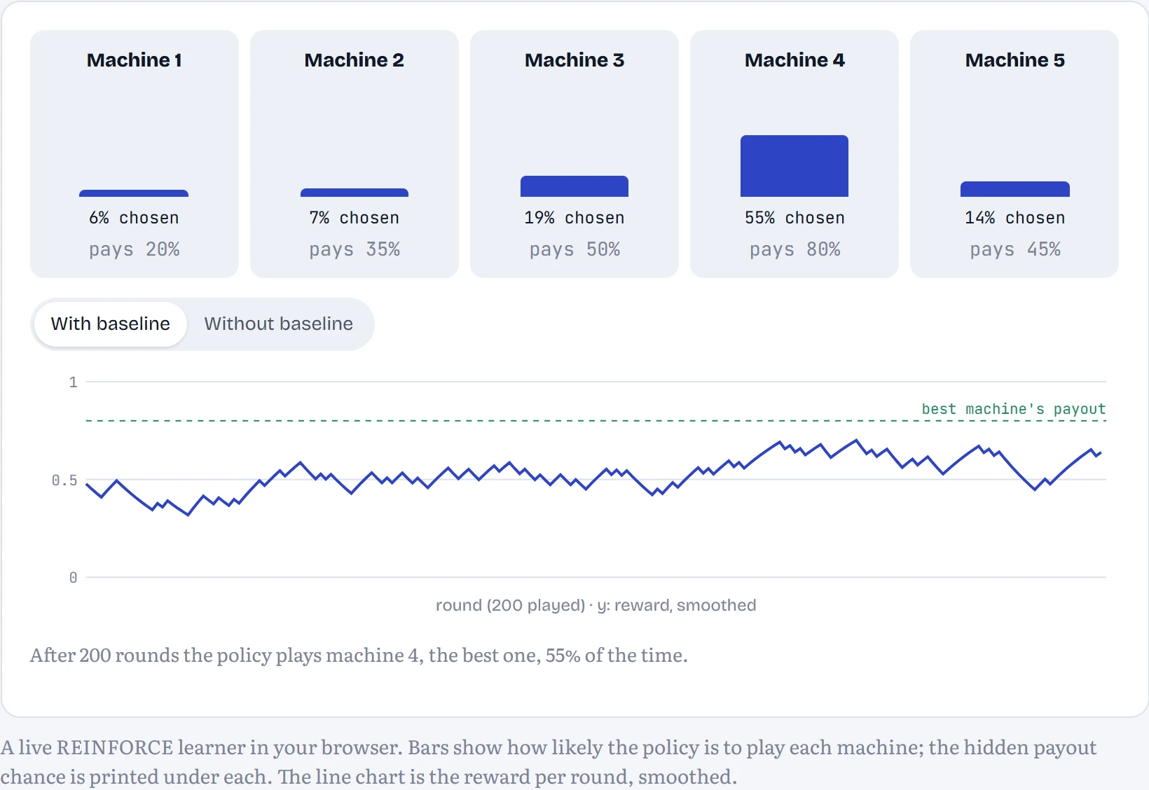
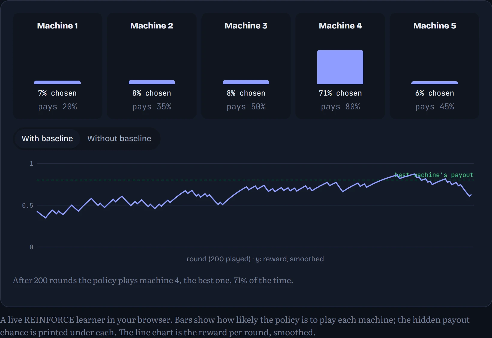
How to read it: at the start, every machine is equally likely. As rounds go by, the bar over the best machine should grow and the others shrink, and the reward line should climb towards the best machine's payout rate. Run it a few times each way. With a baseline, learning is usually faster and steadier; without one, it wanders, because every payout, even from a poor machine, makes that machine more likely.
Large-scale RL for language models adds two safety rails to this idea. PPO (proximal policy optimization) clips each update so a single batch can't change the policy too much. And a KL penalty charges the model for drifting away from where it started, measured as the KL divergence (Chapter 3.3) between the new model's predictions and the original's. You'll see why that second one matters a lot in two sections.
The formal picture: states, actions, rewards, values
RL problems are written down as a Markov decision process (MDP). There are states (where you are), actions (what you can do), transitions (where each action takes you, possibly at random) and rewards. The goal is to maximize the return: the sum of future rewards, each one multiplied by a discount γ (gamma) per step of delay, so that a reward now counts more than the same reward later. The value of a state is the return you can expect from it if you act well from then on. Values obey a simple consistency rule, the Bellman equation: a state's value is the best immediate reward plus the discounted value of where that action leads. Apply that rule to every state over and over and the values settle; that's value iteration.
In the figure: a robot in a small grid. The green square is worth +1, the red one −1, the dark squares are walls, and each move costs the step penalty. With the slip chance, the robot moves sideways instead of where it meant to go. Each square shows its computed value and the best move from it.
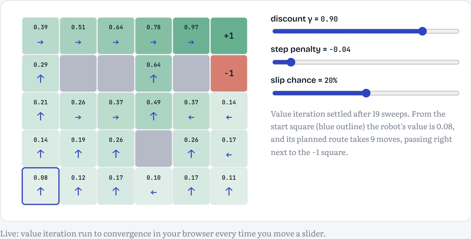
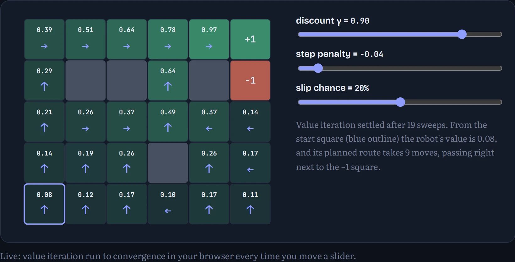
With a large step penalty, the robot heads straight for the exit, risking the red square, because wandering is expensive. With none and a high discount, it takes the long, safe way round. That's the whole point of a value function: it turns a goal that's only rewarded at the end into a judgement about every intermediate state.
For a language model, the MDP is unusually simple and unusually large. The state is the prompt plus every token written so far, the action is the next token (one of ~100,000), the transition is deterministic (the chosen token is appended), and the reward usually arrives only once, when the answer is finished and judged. That last fact makes credit assignment hard: which of the 500 tokens deserved the reward? PPO trains a separate value network to estimate it at every token; GRPO, coming up, avoids the value network by comparing whole answers within a group.
Learning from preferences: RLHF and DPO
For most things people care about in an assistant, like being helpful, clear and honest, there's no formula for the reward. But people can compare: shown two answers to the same question, they can usually say which is better. That's the raw material of RLHF, reinforcement learning from human feedback.
The classic recipe has three steps. First, SFT, as above. Second, collect many comparisons and train a separate reward model to predict them. It uses the Bradley–Terry model: if answer A has score rA and B has rB, the chance a person prefers A is σ(rA − rB), where σ is the sigmoid. Equal scores mean 50/50; a gap of 2 means about 88/12. Third, run RL (usually PPO) against that reward model, with a KL penalty to keep the model close to the SFT version.
DPO, direct preference optimization (Rafailov and colleagues, 2023), gets a similar result with far less machinery. A bit of algebra shows that the optimal KL-penalized policy implies its own reward: β times how much more likely the new model makes an answer than the reference model does. So you can skip the separate reward model and the RL loop, and directly train the model so that, compared with the reference, it raises the probability of the preferred answer more than the rejected one. In code, it's one loss on pairs of answers.
Our preference experiment needed a judge, and to keep it cheap and transparent I wrote one: count the happy words in a story (like smiled, hug, friends) and subtract the sad ones (like cried, scared, alone). Then, for 180 prompts, the SFT model wrote eight stories each; the highest-scoring story became “chosen” and the lowest “rejected”, giving 179 pairs. Here's one:
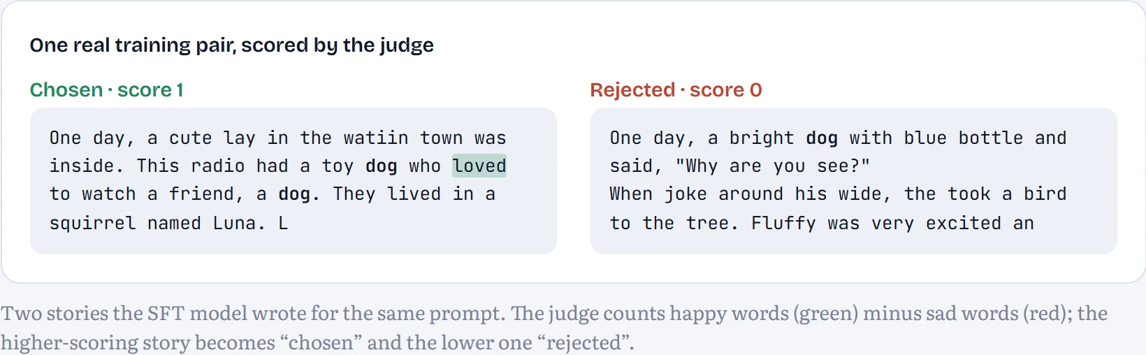
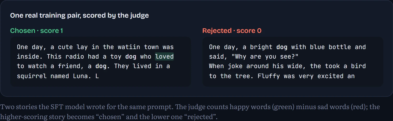
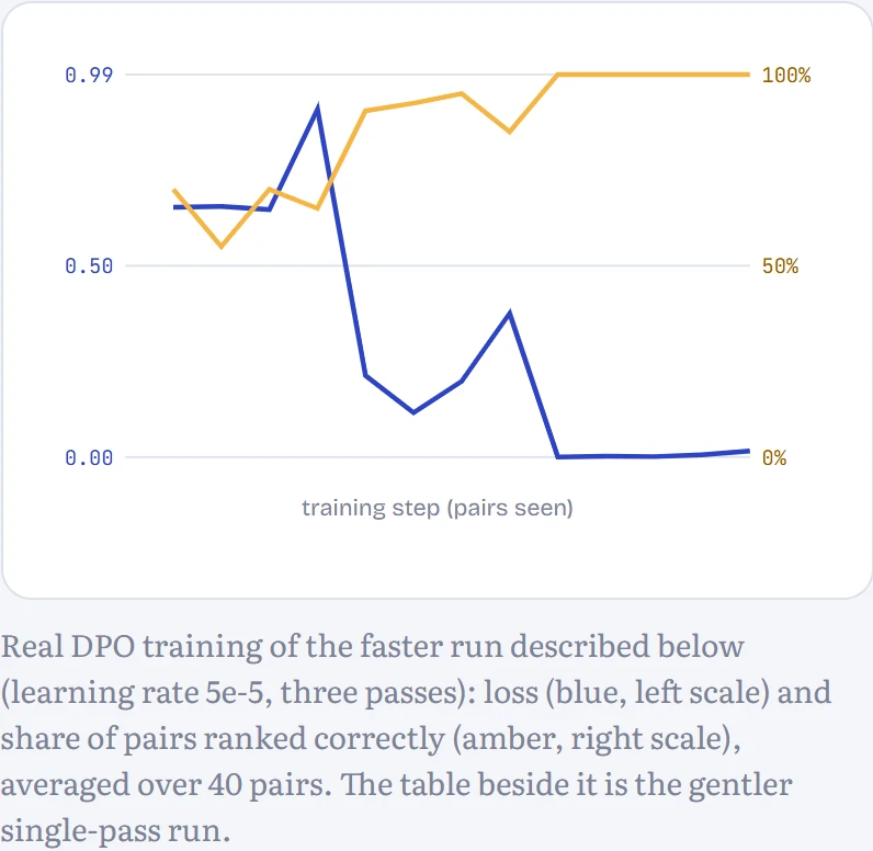
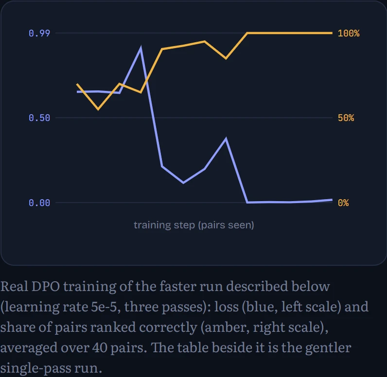
DPO then trained on these pairs. How to read the results: the chart shows the training loss falling and the share of pairs where the model already prefers the chosen story rising. The table compares the model before and after on fresh stories it wasn't trained on: the judge's average score, the share of stories with a positive score, whether it still follows the topic instruction, and its loss on real held-out stories, which tells you whether it's still writing like a storyteller or drifting away.
| Measured on fresh stories | Before (SFT) | After DPO |
|---|---|---|
| Judge's average score | 0.58 | 1.72 |
| Stories scoring above 0 | 52% | 93% |
| Follows the topic | 46% | 42% |
| Loss on real stories | 1.072 | 1.081 |
One pass of DPO moved the judge's average score from 0.58 to 1.72, and the share of stories with a positive score from 52% to 93%, after training on just 179 pairs. Topic-following went from 46% to 42%, and the loss on real stories barely moved. DPO's built-in comparison with the reference model is meant to keep this drift small: it rewards preferring the chosen story more than the reference did, rather than rewarding any change at all.
Too much of a good thing
The gentle result above used a small learning rate (0.00001) and a single pass over the pairs. To see what happens when you push harder, I also trained with five times the learning rate (5e-5) for three passes. How to read the table: each row is that model after one more pass over the same pairs. Watch the judge's score and the loss on real stories move in opposite directions.
Continue the lesson
The whole lesson, with its drawings and its questions. The rest of this section and 6 more after it.