
Distributional semantics: one-hot encoding, co-occurrence matrices, PCA and SVD
A vector is an ordered list of numbers you can read as features, a point or an arrow. Words start as one-hot vectors that say nothing about meaning; counting the company each word keeps turns them into vectors where similar words sit close together, and PCA and SVD compress those into a few dimensions.
What this page answers
What is cosine similarity?
The dot product of two vectors divided by both their lengths. It ignores length and measures only direction: 1 for the same direction, 0 for unrelated and -1 for opposite. Read it in “Vectors: lists, arrows and points”
Why multiply a one-hot vector by a matrix?
Multiplying a one-hot vector by a matrix picks out one row of it. That lookup is the seed of an embedding table, where each word's row is its learned vector. Read it in “One-hot × matrix: the seed of embeddings”
Vectors: lists, arrows and points
A vector is just an ordered list of numbers, like [3, 1]. You can read the same list in three ways, and switching between them is half of linear algebra. It's a list of features (a house's [size, rooms]). It's a point in space (3 across, 1 up). And it's an arrow from the origin to that point, with a length and a direction. The number of entries is its dimension: [3, 1] is 2-dimensional, a 28 × 28 image flattened into a list is 784-dimensional, and the word vectors in this lesson have 50 dimensions. You can't picture 50 dimensions, but every rule below works the same in 2 as in 50 or 12,288.
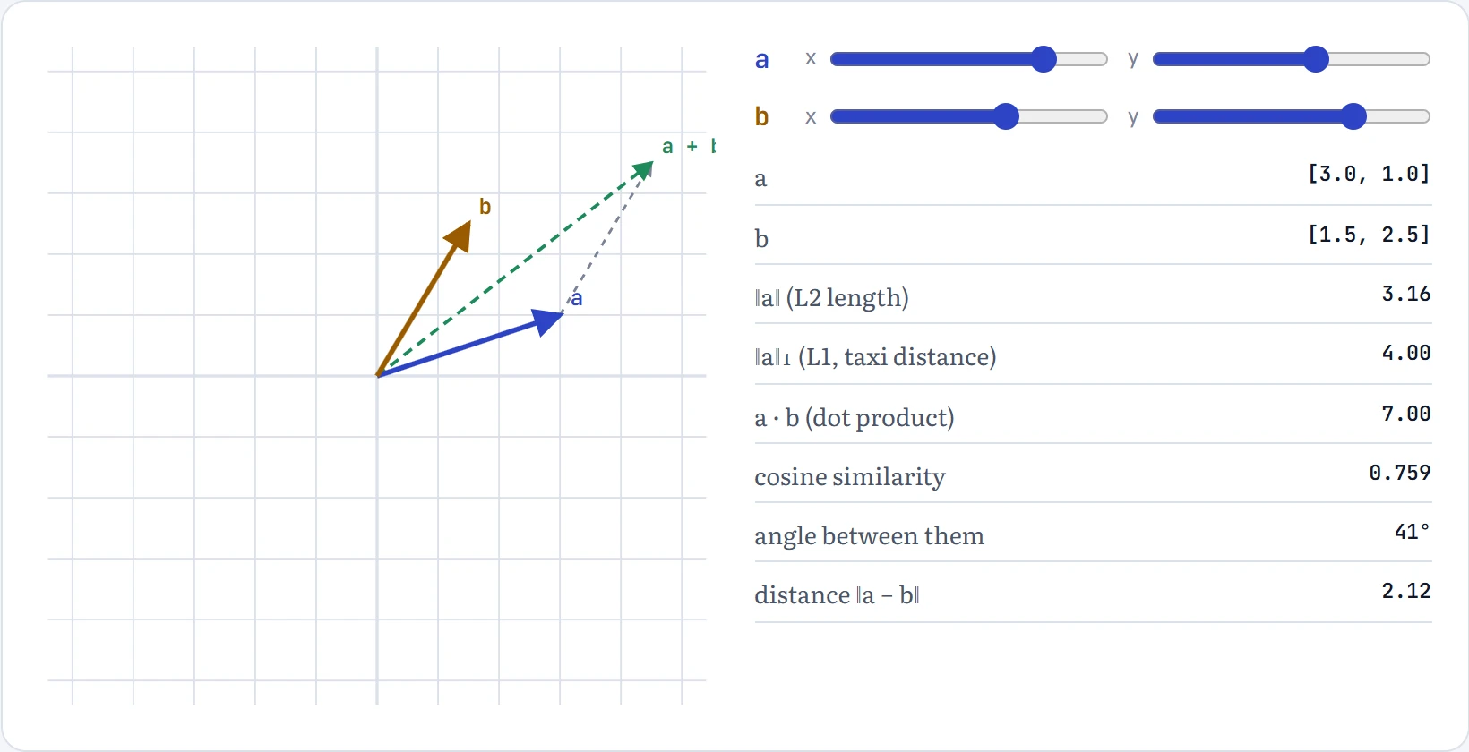
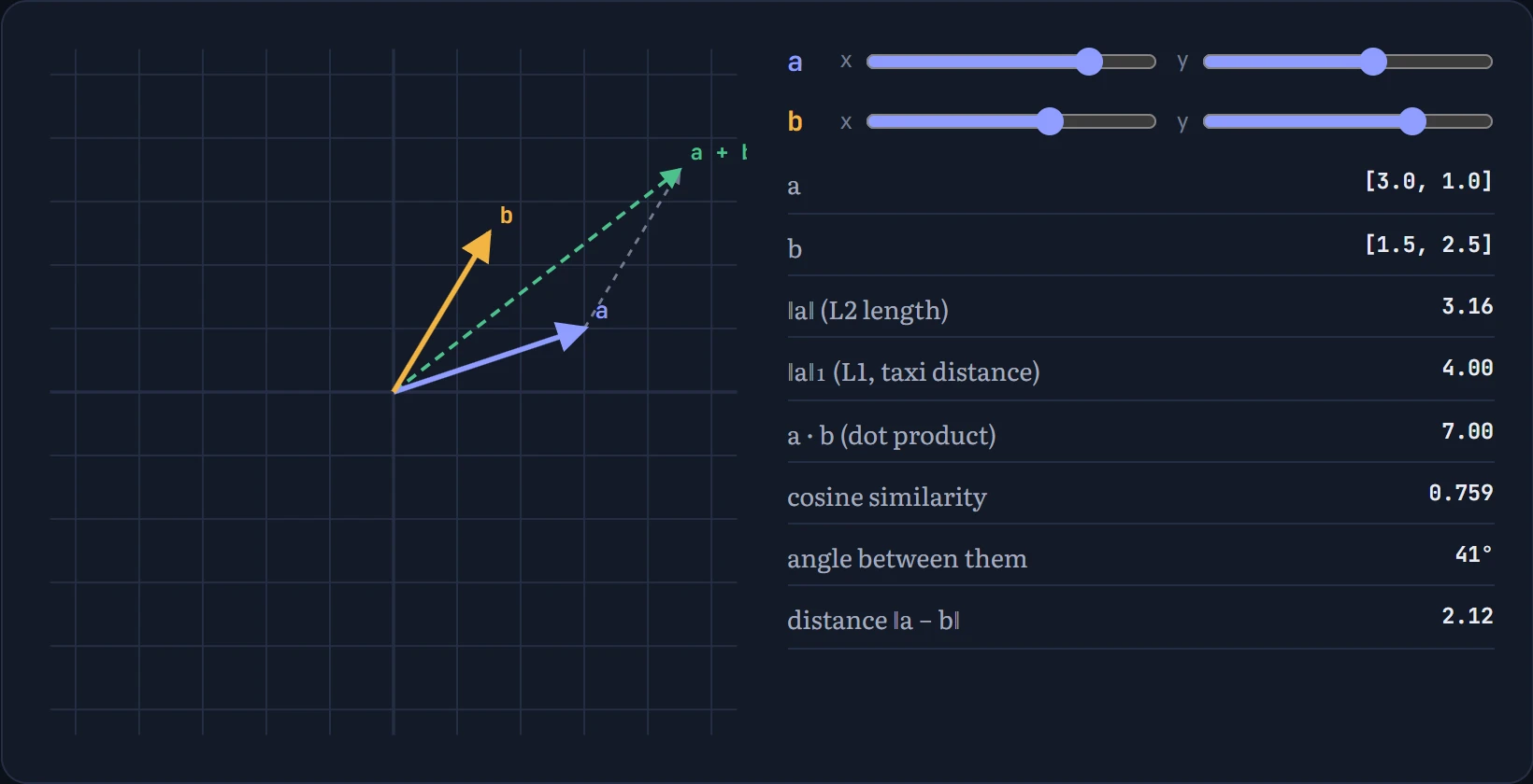
The length of a vector is its norm. The usual one, the L2 norm, is Pythagoras: ‖a‖ = √(a₁² + a₂² + …). The L1 norm adds absolute values instead (the distance a taxi drives on a grid). Comparing two vectors uses the dot product, a · b = a₁b₁ + a₂b₂ + …: multiply matching entries and add. It's large when the vectors point the same way, zero when they're at right angles, and negative when they point apart. Divide it by both lengths and you get the cosine similarity, which ignores length and measures only direction: 1 for the same direction, 0 for unrelated, −1 for opposite. In the figure: two arrows, with every quantity computed from them.
Words as one-hot vectors
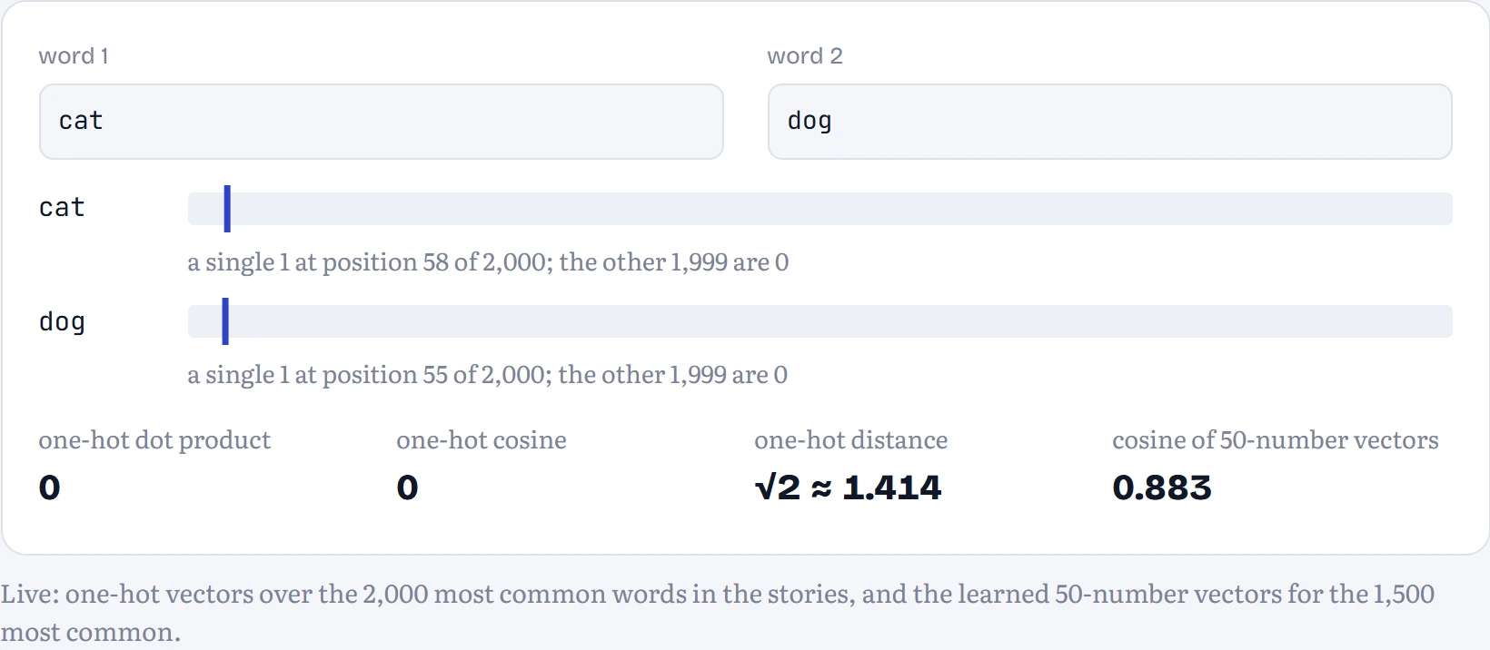
The simplest way to turn a word into a vector: give every word in the vocabulary a number, then represent word number i as a vector of zeros with a single 1 in position i. That's a one-hot vector. With our 2,000-word vocabulary, “cat” is 2,000 numbers, all zero except one. Your Chapter 1 bigram did exactly this with characters, and so does the input of every language model before anything clever happens.
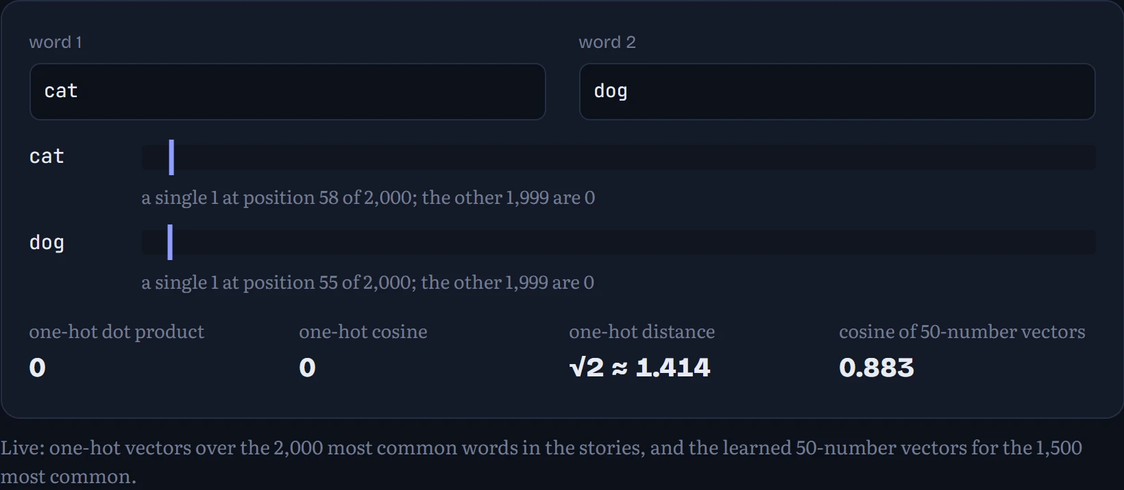
One-hot vectors are honest but useless for meaning. Any two different one-hot vectors have a dot product of 0 and a distance of √2, so as far as the vectors are concerned “cat” is exactly as similar to “dog” as it is to “spoon”. In the figure: two words. The strips show where each one-hot vector's single 1 sits among its 2,000 positions; underneath, their similarity as one-hot vectors, and as the 50-number vectors we'll build later in this lesson.
Predict first. Using one-hot vectors, what's the cosine similarity between “happy” and “glad”? And between “happy” and “happy”?
- High, then 1
- 0, then 1
- 0.5, then 1
Answer. 0 and 1. One-hot vectors only know whether two words are the same word. Every different pair scores exactly 0, synonyms included. To capture meaning, the numbers themselves have to carry information, which means we need to learn them from data.
Meaning from the company a word keeps
Where would better numbers come from? Linguists in the 1950s proposed an answer that turned out to be the foundation of modern AI: words that appear in similar contexts have similar meanings. J. R. Firth's version: “You shall know a word by the company it keeps.” This is the distributional hypothesis. You've never been told that “cat” and “dog” are alike, but you've seen both after “the”, both before “was sleeping”, both near “fed” and “pet”.
So let's count company. For every word in 20,000 stories (3.2 million words), I counted how often each of the 2,000 most common words appeared within four words of it. The result is a 2,000 × 2,000 co-occurrence matrix: one row per word, and that row is a 2,000-number vector describing its company. How to read the table: a few real rows and columns of it. Look at how the rows for cat and dog resemble each other, and how happy and sad share “felt” and “very”.
| word ↓ / near → | the | a | was | played | felt | food | fast | very |
|---|---|---|---|---|---|---|---|---|
| cat | 10,162 | 4,556 | 2,873 | 213 | 112 | 91 | 72 | 484 |
| dog | 9,101 | 4,799 | 2,956 | 255 | 93 | 62 | 115 | 444 |
| happy | 8,281 | 2,019 | 11,288 | 858 | 1,116 | 86 | 53 | 4,802 |
| sad | 3,225 | 639 | 4,750 | 9 | 1,231 | 20 | 25 | 1,341 |
| ate | 1,035 | 115 | 169 | 136 | 52 | 173 | 18 | 77 |
| ran | 3,213 | 409 | 575 | 102 | 41 | 4 | 351 | 228 |
Two things jump out. Cat and dog have nearly the same pattern (10,162 and 9,101 times near “the”, 213 and 255 near “played”), while happy and sad share a quite different one, with lots of “felt” (1,116 and 1,231) and “very”. That's the distributional hypothesis, visible in raw numbers. The second thing is a problem: the column for “the” dwarfs everything, because “the” is near almost every word. If we compared rows directly, every word would look similar to every other word simply for sharing “the”. Two standard fixes: compare directions with cosine similarity rather than raw dot products, and shrink big counts by taking their logarithm, log(1 + count), so 10,000 becomes about 9.2 and 100 becomes about 4.6.
A space of words
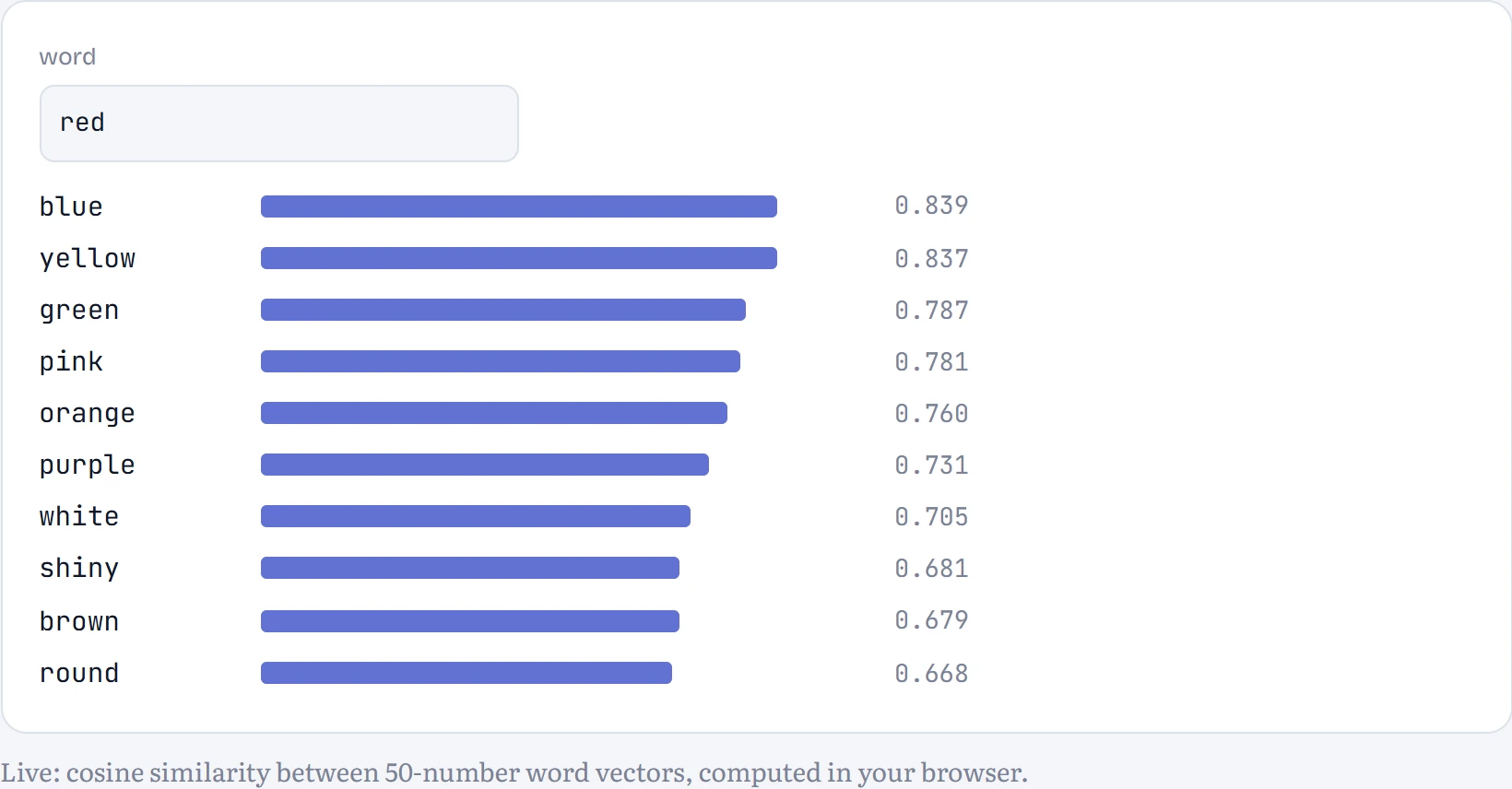
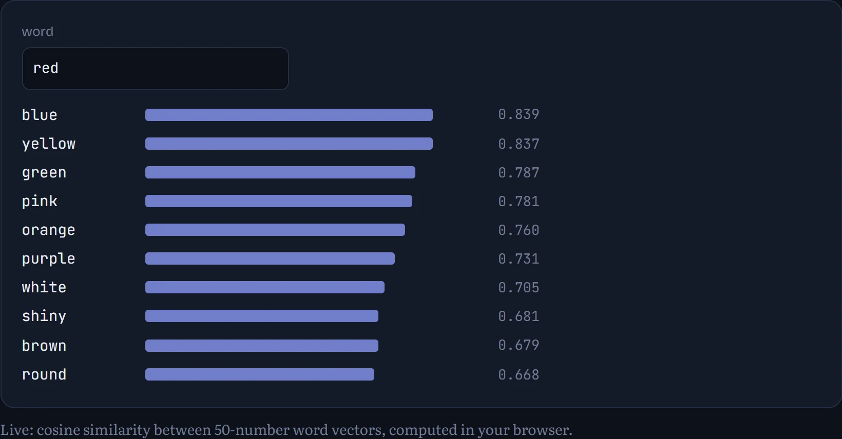
Each word is now a point in a space, and similar words should be near each other. Later in this lesson we'll compress those 2,000-number rows down to 50 numbers per word with a technique called SVD (and see what that compression keeps and what it loses). For now, try the result. In the figure: a common word; the list shows its nearest neighbours by cosine similarity among the 1,500 most common words, with the similarity score.
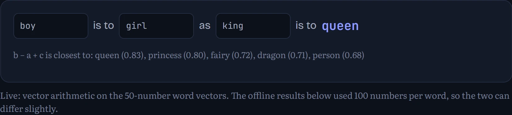
The vectors also have structure in their directions. If the difference between “boy” and “girl” is a consistent direction in the space, then king − boy + girl should land near queen. That's an analogy by vector arithmetic, made famous by word2vec in 2013. In the figure: an analogy, a is to b as c is to ?: the demo computes b − a + c and lists the nearest words (excluding the three given).
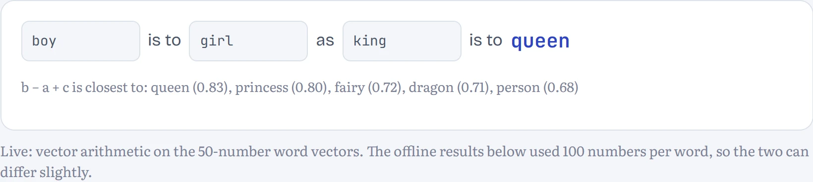
Here's how seven classic analogies came out (100 numbers per word): boy : girl :: king : queen; man : woman :: prince : princess; mom : dad :: mommy : daddy; big : bigger :: small : stronger; cat : kitten :: dog : puppy; walk : walked :: run : ran; one : two :: three : five. 5 of 7 are what a person would say. The misses are instructive: small → “stronger” (with “smaller” second) and three → “five” (with “four” second). The vectors know these words belong to the right family, but the step from “big” to “bigger” isn't a perfectly consistent direction in a model built from 3 million words of children's stories. Analogies make a great demo; researchers have since shown they're a fragile test of word vectors, so treat them as a probe, not a score.
Matrices transform space
A matrix is a grid of numbers, and its most important job is to transform vectors. Multiplying a matrix by a vector means taking the dot product of each row with the vector: a 2 × 2 matrix [[a, b], [c, d]] sends [x, y] to [ax + by, cx + dy]. Every neural network layer you'll meet is mostly this, a matrix multiplication followed by a small nonlinear step, so it pays to see what one does. The trick is to watch what happens to the whole grid, not one point. In the figure: a 2 × 2 matrix. The faint grid is the original space, the blue grid is where the matrix sends it, and the F shows orientation.
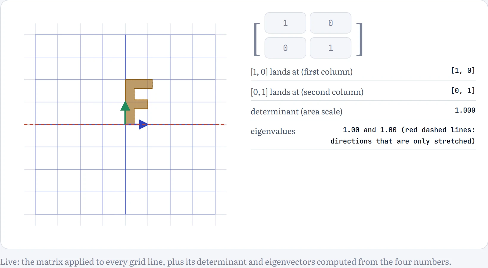
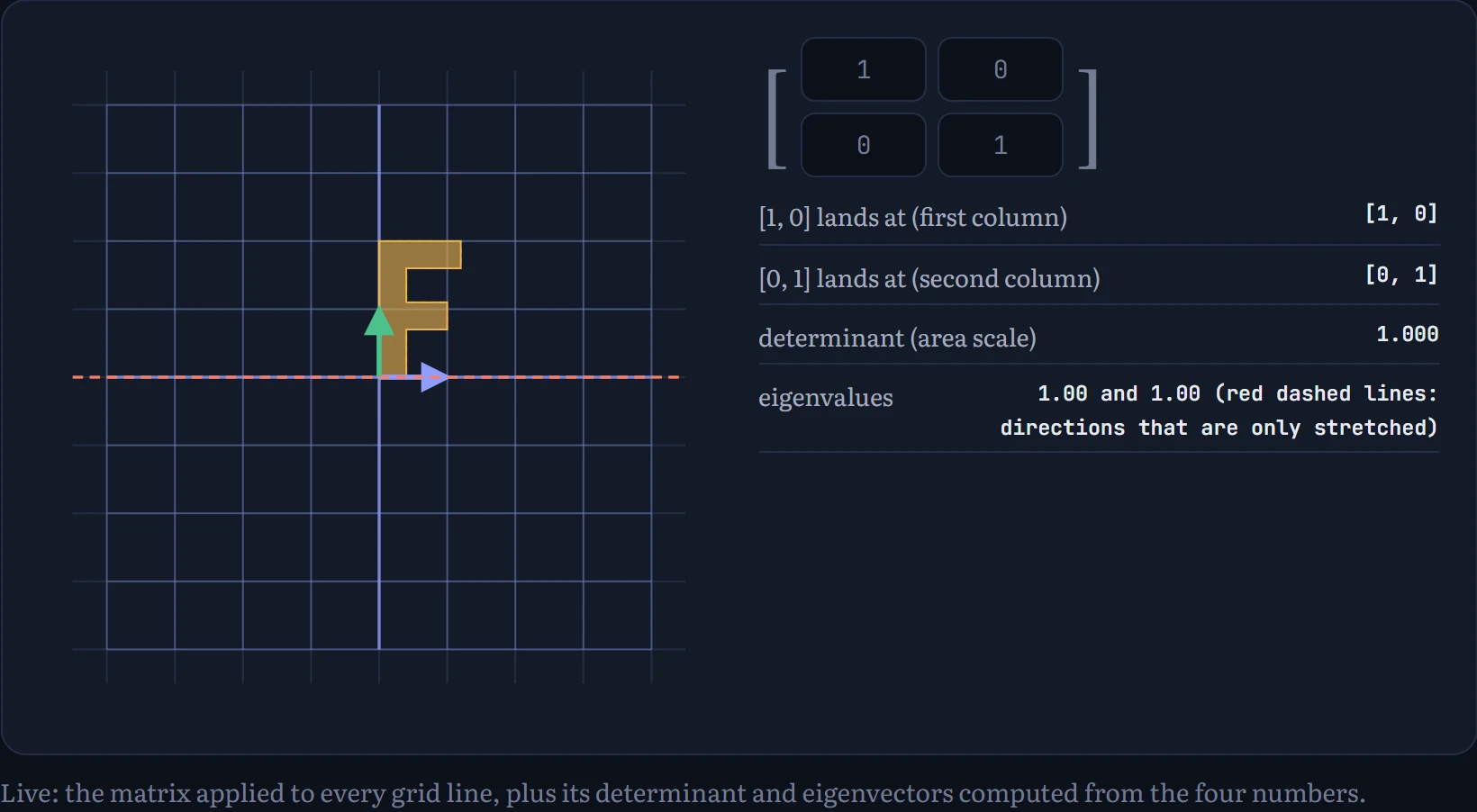
Three ideas to take away. The first column of the matrix is where the arrow [1, 0] lands, and the second column is where [0, 1] lands; everything else follows, because the transformation keeps grid lines straight, parallel and evenly spaced (that's what linear means). The determinant is how much areas grow: 2 means doubled, 0 means the whole plane was squashed onto a line, and negative means the plane was flipped over. And an eigenvector is a direction that the matrix only stretches, without turning; the stretch factor is its eigenvalue. In a shear, one direction stays put while everything else slides along it. A matrix that squashes the plane onto a line has rank 1: its output only uses one dimension's worth of space. Rank will come back when we compress the word matrix.
Multiplying two matrices, AB, means doing B's transformation and then A's. Each entry of the product is a dot product of a row of A with a column of B, so an (m × n) matrix times an (n × p) matrix needs m × n × p multiply-adds and gives an m × p result. The inner sizes must match. That one rule explains most of the shape errors you'll ever see.
One-hot × matrix: the seed of embeddings
Here's the connection to your bigram model. Store its counts as a matrix M, one row per current character, one column per next character, each row normalized to add up to 1. Now multiply a one-hot vector for “t” by M. Every term of each dot product is zero except the one where the 1 sits, so the result is simply row t of M: the probability of each next character after “t”. A one-hot vector times a matrix is a lookup. In the figure: one character. The highlighted row of the matrix is what the multiplication picks out, and the bars are that row.
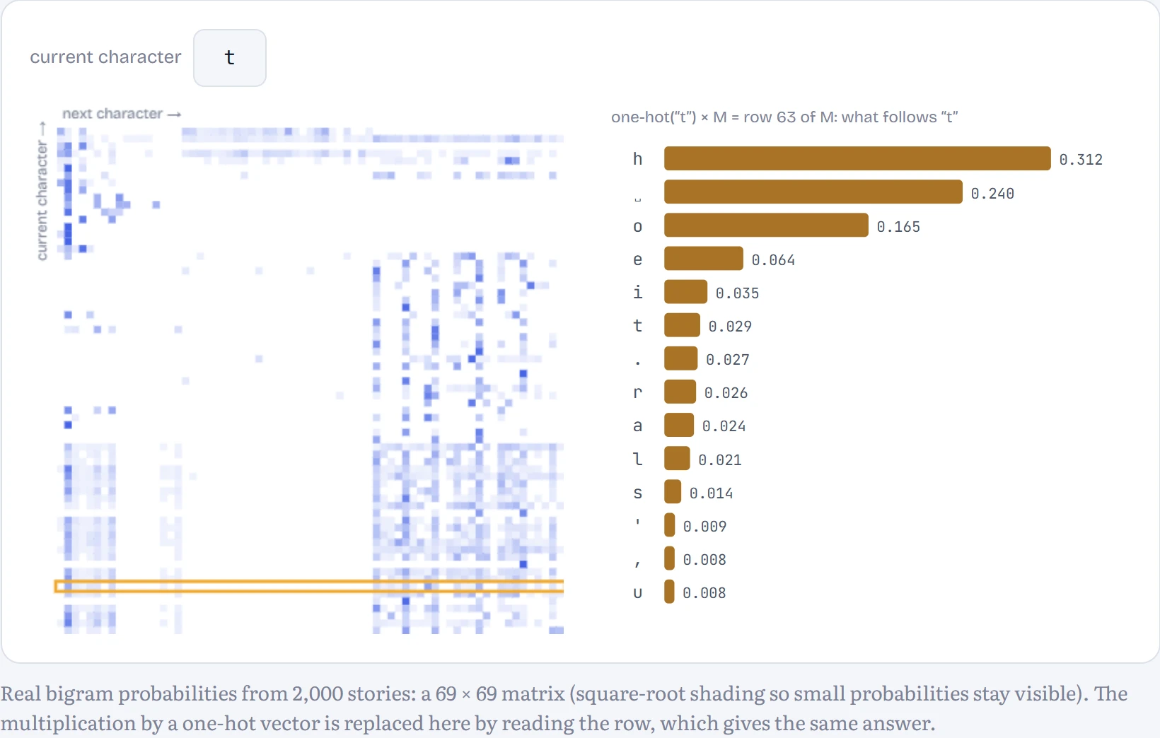
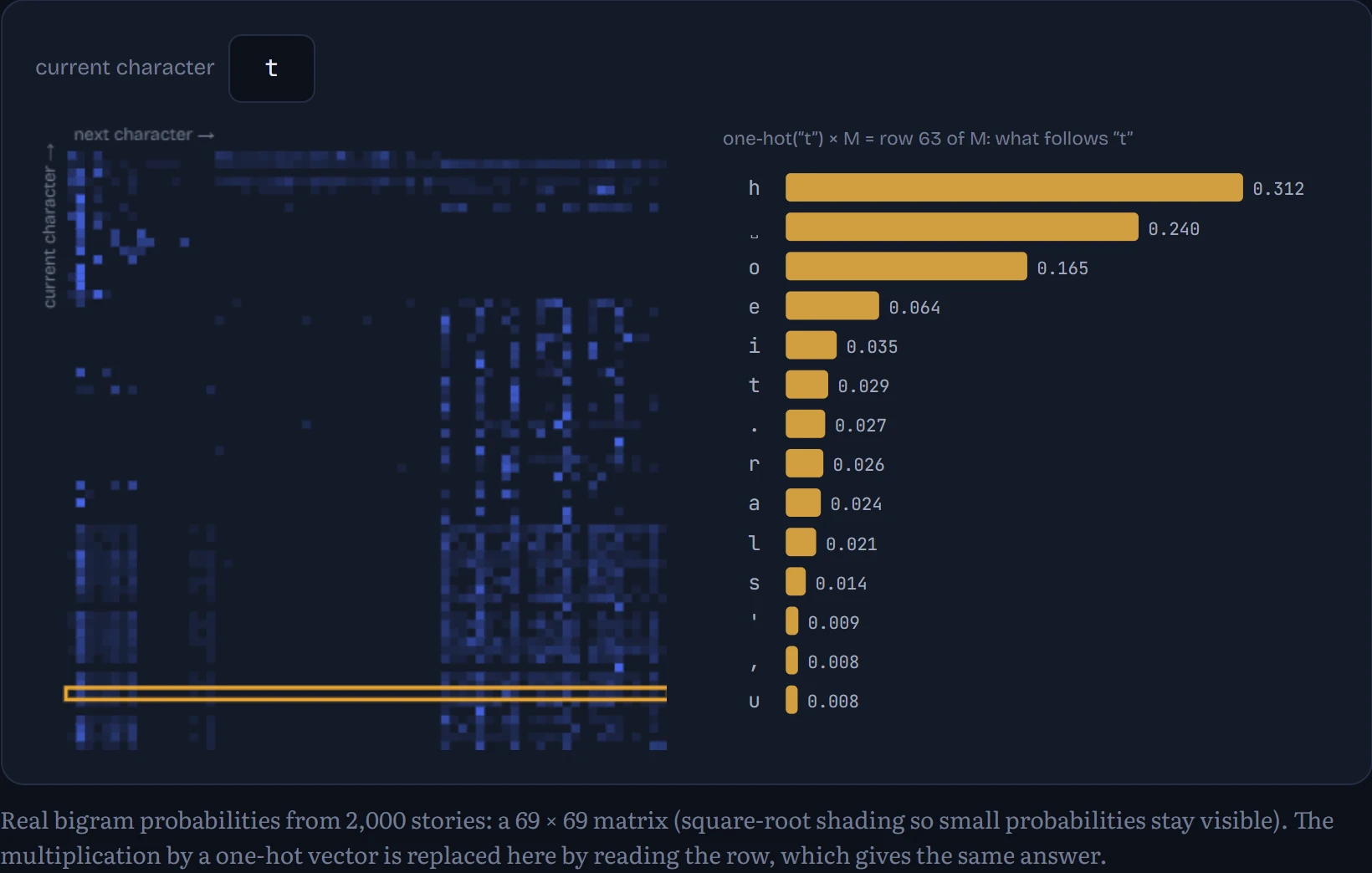
That's why the first layer of every language model is called an embedding. Instead of a row of next-character probabilities, each token's row holds a short learned vector, say 50 or 4,096 numbers, and multiplying the one-hot input by that matrix just looks the vector up. Libraries skip the multiplication and index the row directly, but it's the same operation, and it's why gradients can flow into the table: the lookup is a matrix product, so calculus applies. You'll train one in Chapter 6.
Tensors, shapes and speed
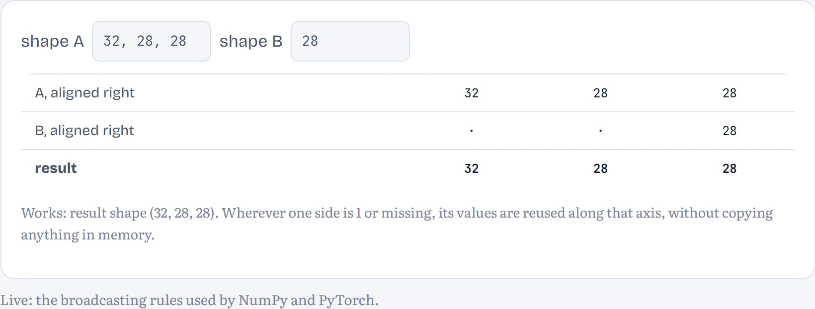
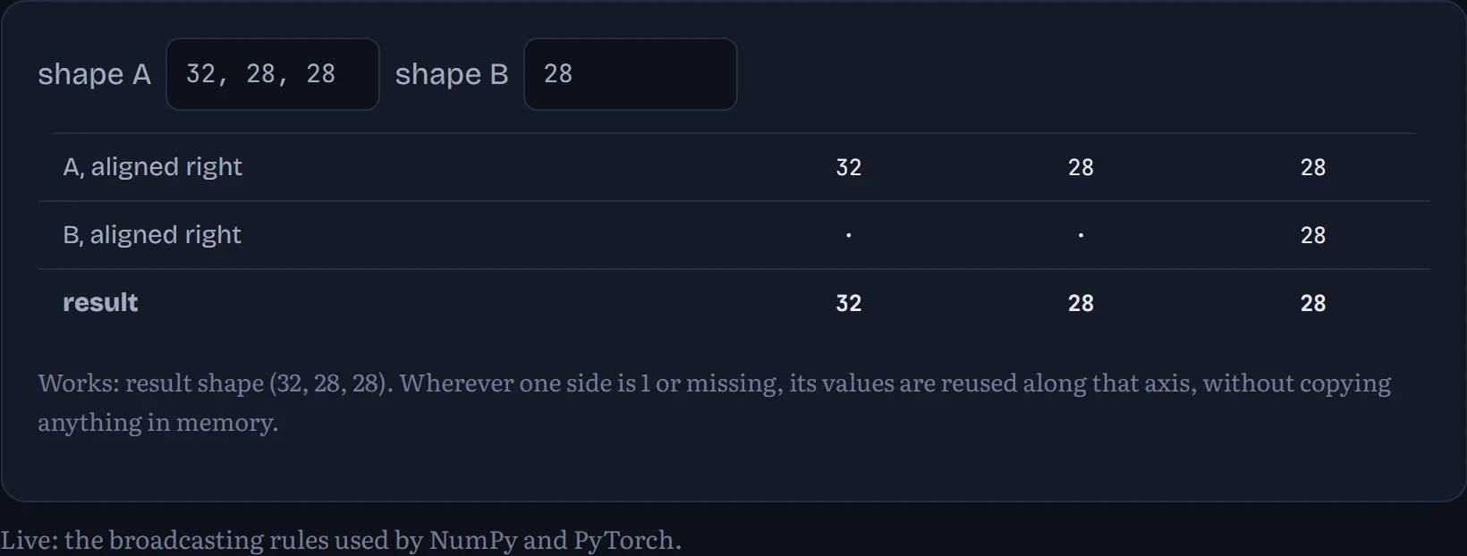
A tensor is the same idea with any number of axes: a single number has 0 axes, a vector 1, a matrix 2, and a batch of 32 colour images of 224 × 224 pixels is a 4-axis tensor of shape (32, 3, 224, 224). Libraries like NumPy and PyTorch do arithmetic on whole tensors at once, and when two tensors have different shapes they broadcast: line the shapes up from the right; at each position the sizes must match, or one of them must be 1 (which gets stretched to fit), or missing. In the figure: two shapes, and whether they combine, and into what.
Why insist on whole-tensor operations instead of writing loops? Speed, by an absurd margin. I timed the same computations three ways on this laptop: plain Python loops, NumPy, and PyTorch. How to read the chart: billions of multiply-adds per second (GFLOP/s, log scale) for multiplying two n × n matrices; higher is faster. Python loops were only timed up to n = 128, because beyond that they take too long to bother.
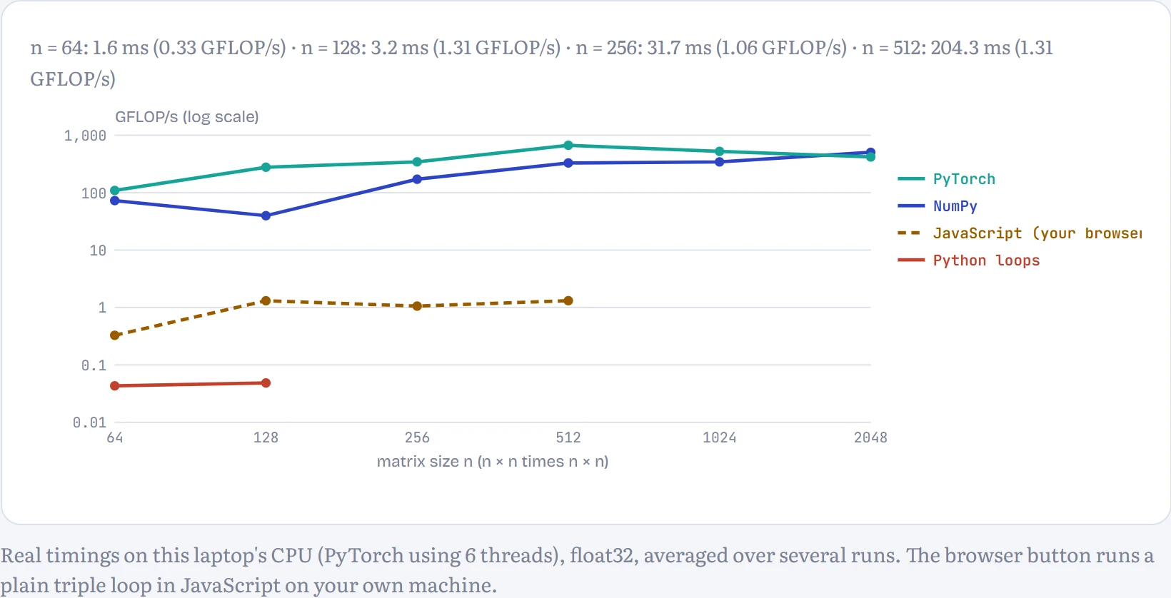
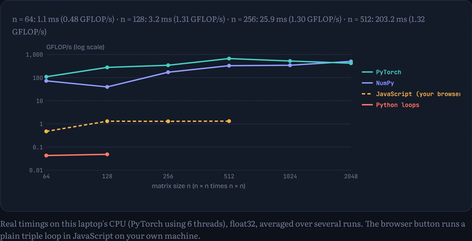
Python loops manage about 0.05 GFLOP/s, because every single multiply goes through the interpreter's bookkeeping. NumPy and PyTorch hand the whole matrix product to compiled code that uses the processor's vector instructions and all its cores, reaching 504 and 419 GFLOP/s at n = 2,048. At n = 128 PyTorch was 5,727 times faster than the loops. The same holds for a simple dot product of two million-number vectors: 26 ms in a Python loop, 0.16 ms in NumPy. Note also that small matrices run slower per operation than big ones: there's a fixed cost per call, and big products keep the hardware busier.
That's the case for batching too. Running a 1,024 × 1,024 layer on one example at a time cost 23.9 microseconds per example; feeding 256 examples at once as one matrix product cost 5.3, about 4 times cheaper per example. (Timings this short are noisy: across three runs on the same laptop the saving ranged from 2 to 11 times, but batching won every time.) A GPU takes this to the extreme: thousands of simple cores that do almost nothing but multiply-adds, which is exactly what matrix products need. That's why AI hardware is built around matrix multiplication, and why the whole field writes its models as operations on tensors.
Continue the lesson
The whole lesson, with its drawings and its questions. 5 more sections after the ones above.