
Bigram language models: count-based estimation, sampling, smoothing and perplexity
A bigram model counts which word follows which in a large body of text, then predicts the next word from those counts. Generating text is a loop: pick a likely next word, append it, repeat. Perplexity measures how surprised the model is by new text, so a lower number is a better model.
What this page answers
What is a bigram language model?
A model that predicts the next word from the one word before it, using a table of how often each pair of neighbouring words appeared in its training text. Read it in “Counting pairs: the bigram model”
Is next-word prediction how chatbots write text?
Yes. At heart, large chatbots produce text the same way: guess the next piece of text, add it, and guess again. The bigram model is the smallest version of that machine. Read it in “Rules, or learning from examples?”
Rules, or learning from examples?
There are two ways to make a computer do something clever. You can write rules: “if the email contains ‘you have won’, mark it as spam.” That works until spammers write “you've won”, and then you need another rule, and another, forever. Or you can show the computer thousands of examples, emails already marked spam or not, and let it work out the patterns itself. That second approach is machine learning, and it's what “artificial intelligence” almost always means today. Not a mind, but a system whose behaviour comes from data instead of from rules someone typed in.
Every learning system has inputs (what it's given), outputs (what it produces) and a task that connects them. Ours is the task behind every chatbot: the input is some text, the output is a guess at the next word. Try it yourself first.
Predict first. In a big collection of children's stories, what word most often follows “Once upon a”?
- time
- hill
- day
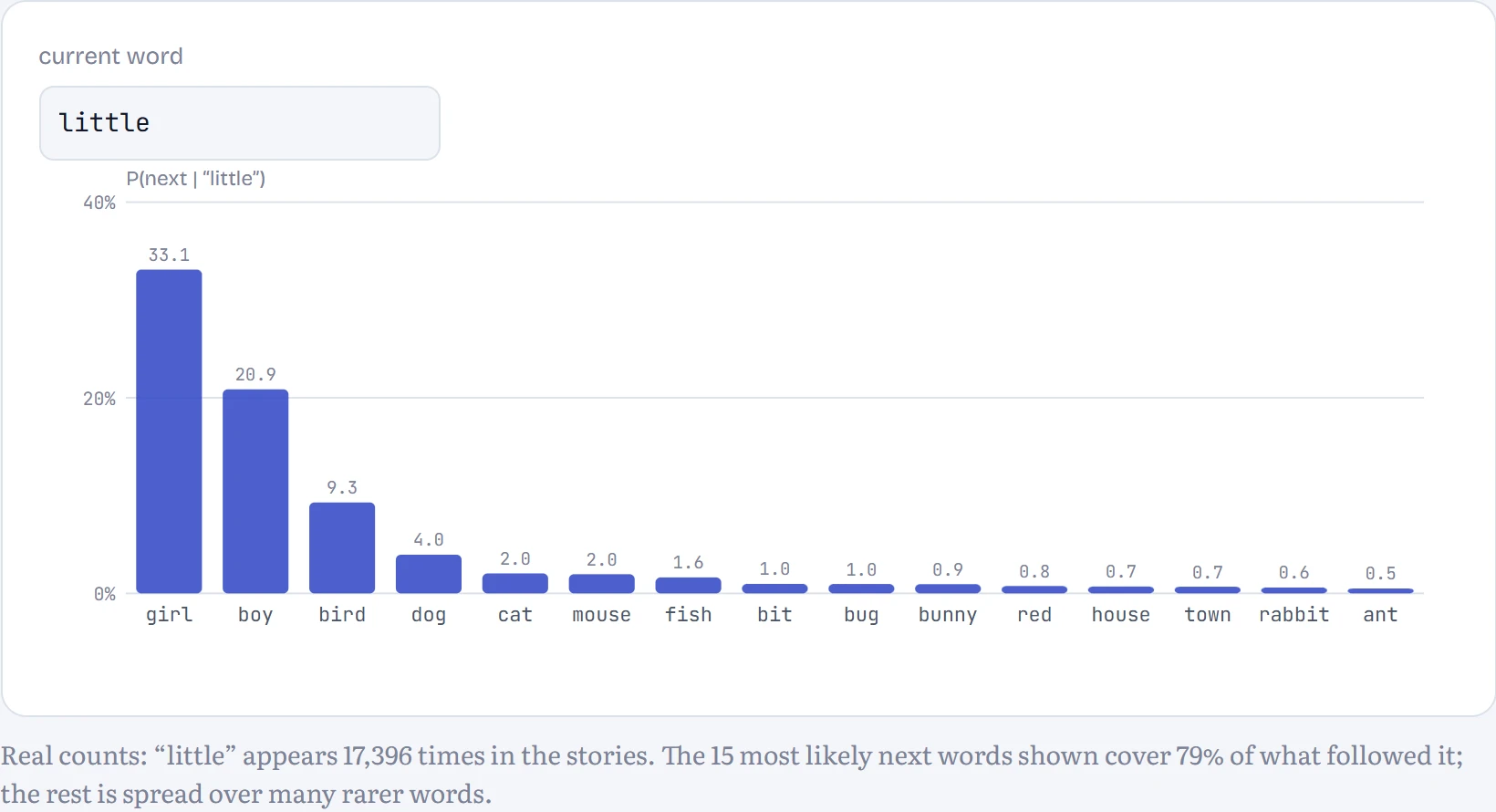
Answer. “time”, overwhelmingly: “once upon a time” opens thousands of the stories. But notice something about the model we're about to build. It only ever looks at the single previous word. After “upon” it's sure the next word is “a” (99.9%). After “a”, though, it has forgotten the “once upon” and gives “time” only about 11%: “a” is followed by hundreds of different words. You used three words of context; it uses one. Keep that in mind; it's the theme of the whole chapter.
You just did what our model will do: you've seen “once upon a time” so often that “time” feels inevitable. Nobody gave you a rule. Your phone keyboard does the same when it suggests the next word. In the lesson, a demo suggests the three words that most often came next in 20,000 stories, after the last word typed.
Here's the surprising part: that is, at heart, how ChatGPT, Claude and Gemini produce text. They take everything written so far, compute a probability for every possible next word (or piece of a word, called a token), pick one, add it to the text, and repeat. How to read the diagram: the loop every one of them runs, once per token.
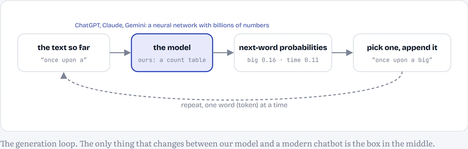
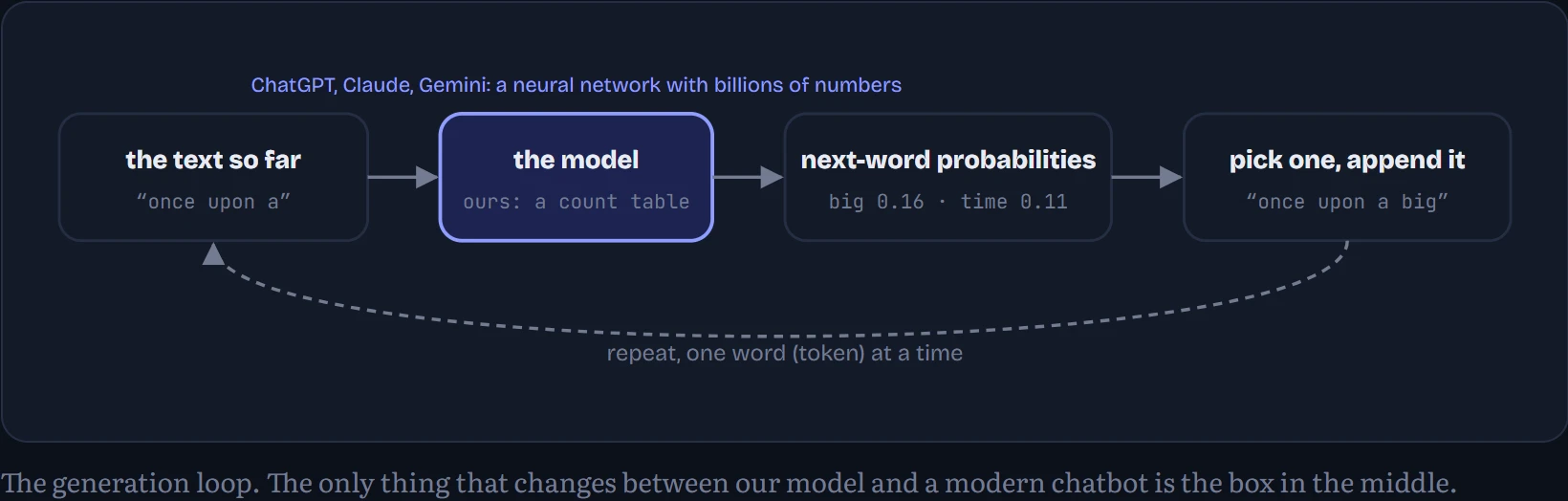
What's in the box makes all the difference. Ours will look at one previous word and consult a table of counts. A modern model looks at thousands of previous tokens through billions of learned numbers, and was then trained further to follow instructions and be helpful. But the outside of the machine, text in, next-token probabilities out, repeat, is the same. This course builds that box from the inside, starting today with the simplest version that works at all.
From words to numbers
Computers only work with numbers, so the first step is always the same: chop the text into pieces and give each distinct piece an ID number. The pieces can be single characters (letters, spaces, punctuation) or whole words. The list of all distinct pieces is the vocabulary. In the figure: text turned into IDs both ways. Word IDs are ranks: 1 is the most common word in the stories.
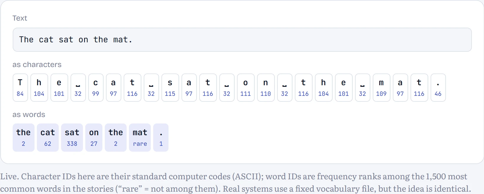
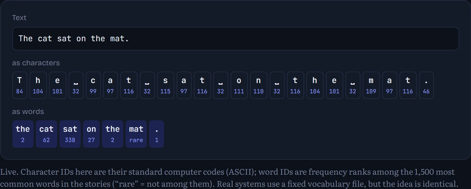
Which pieces should we use? Our 20,000 stories contain 15,985,808 characters but only 76 different ones, so a character vocabulary is tiny. Split into words instead and there are 3,815,962 words but 9,734 different ones, and 2,376 of those appear only once. Words carry more meaning per piece; characters never meet a piece they don't know. Modern models use something in between, chunks of words called tokens, which Chapter 6 builds.
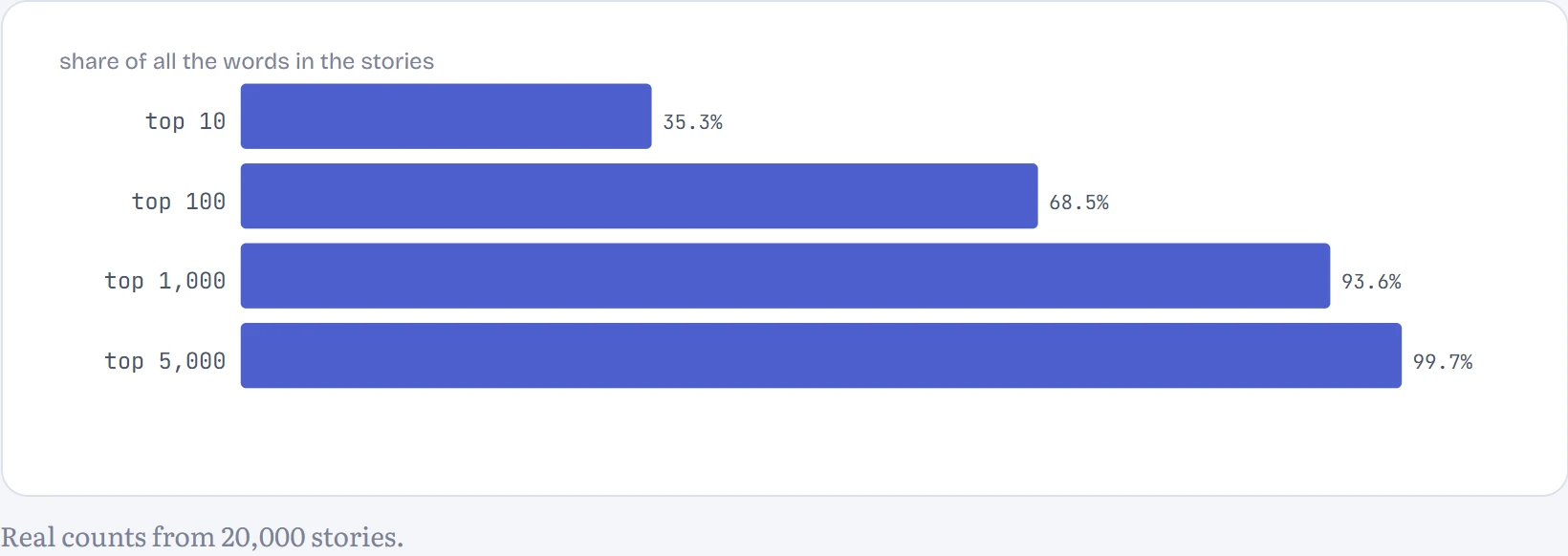
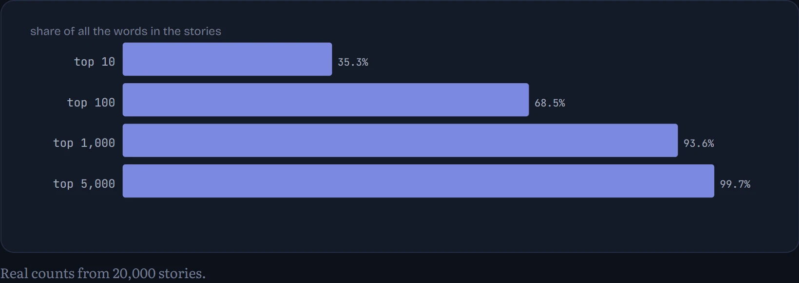
Word counts are wildly uneven. The most common pieces are “.” (322,040), “the” (195,893), “,” (174,899), “and” (145,719), “a” (111,926), “to” (109,142), “"” (86,268), “was” (78,035). How to read the chart: the share of all the text you'd cover if your vocabulary held only the most common 10, 100, 1,000 or 5,000 words.
Now the question that drives the whole chapter. If someone says “I am”, what comes next? How to read the chart: the words that followed “am” in the stories (left) and the words that followed the two-word phrase “I am” (right), as a share of all the times each appeared.
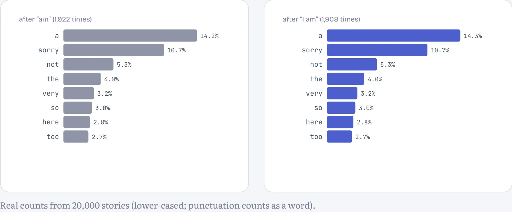
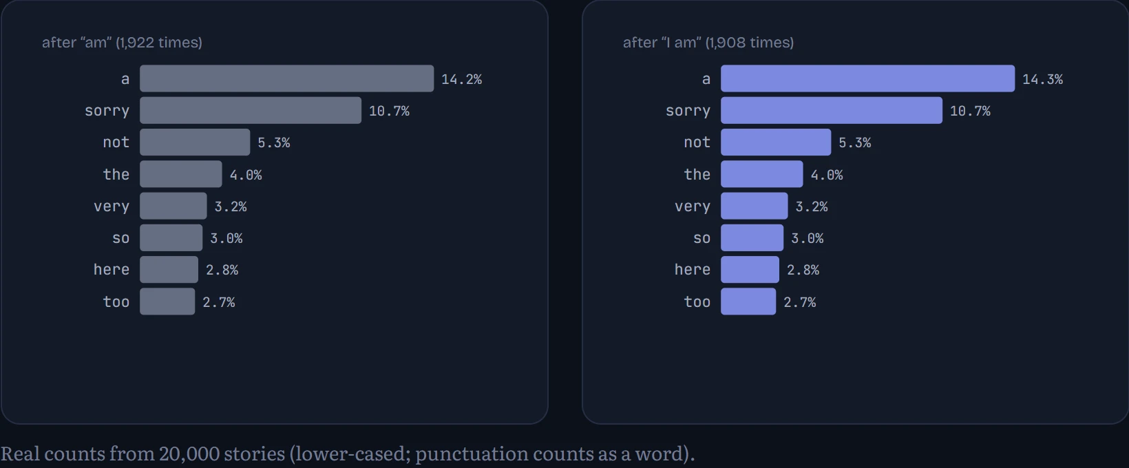
The most common continuation of “I am” is “a” (14%), then “sorry” (11%): children's stories are full of apologies. The two charts differ because one extra word of context changes the odds; that's the theme we'll keep coming back to. Either way, the machine's answer is never one word. It's a distribution: a list of possible next words, each with a probability. Turning counts into such lists is the next step.
Counting pairs: the bigram model
Here's the whole model. Go through the text and, for every word, note which word came right after it. Keep a tally for every pair. A pair of neighbouring words is a bigram (“bi” for two), so the tally is a bigram table: one row for each word, one column for each word that might follow it. Let's do it by hand on three tiny sentences.
To turn counts into predictions, divide each count by its row total. That gives a probability, a number between 0 and 1 saying how often something happens, written P(next | current) and read “the probability of the next word, given the current one”. In the hand example, “like” was followed by “cats” twice and “dogs” once, so P(cats | like) = 2/3 and P(dogs | like) = 1/3. Each row's probabilities add up to 1: something has to come next.
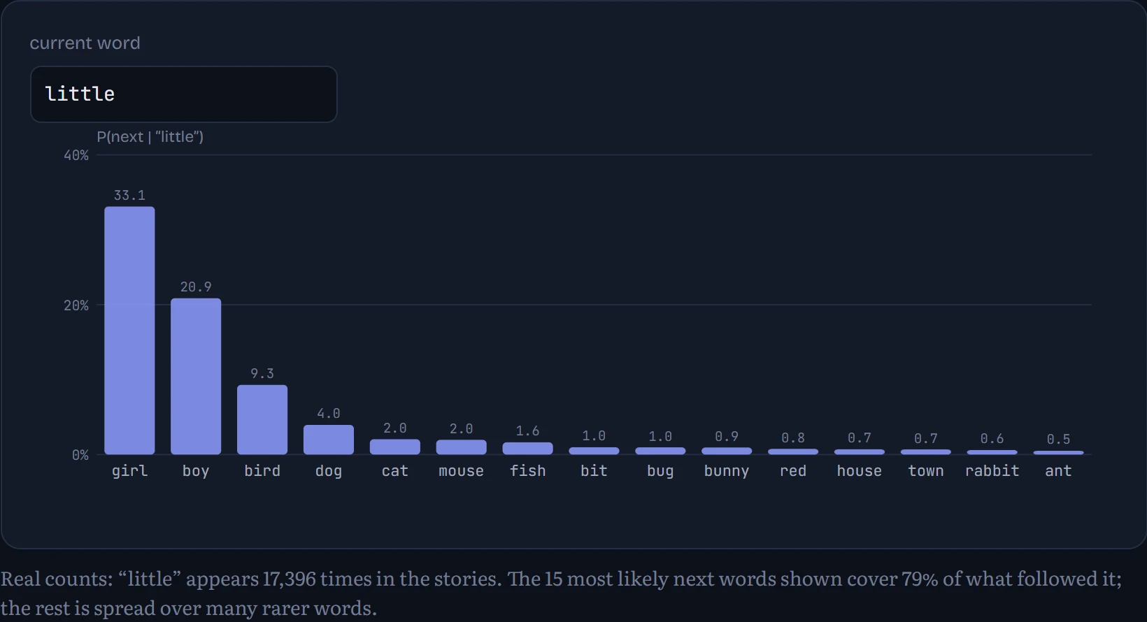
Now the real thing: the same counting, done on 3.8 million words of stories. Below, a word and the words that follow it, as probabilities.
Predict or sample: generating text
To generate text, run the loop: look up the last word's row, choose a next word, append it, repeat. There are two ways to choose. Predicting (also called greedy decoding) always takes the single most likely word. Sampling rolls a weighted die: a word with probability 0.3 is chosen 30% of the time. In the figure: a starting phrase, continued both ways. Sampling gives a different continuation each time; greedy gives the same one every time.
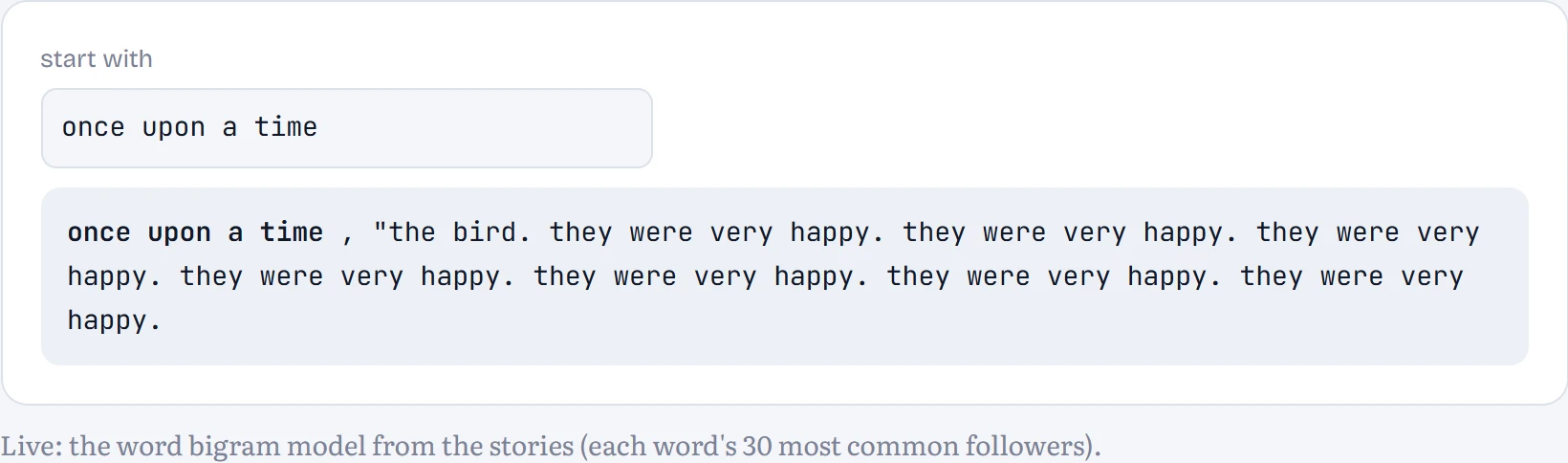
Greedy decoding gets stuck almost immediately. From “once upon a time” the most likely path runs: once upon a time, "the bird. they were very happy. they were very happy. they were very happy. they were very happy. It goes round in that circle forever, because once it reaches “they”, the most likely continuation is always the same, and the model remembers nothing older than one word. Sampling never repeats exactly, and every phrase in it is locally plausible, yet the whole is nonsense. Here are two samples from the Python run: “once upon a time, making you are a red wagon together, "now we do anything. then, cars later, "her shovel. the store. the yard.”, “once upon a time and rocks and promised not too late. they could fit in the birds, changing, the shop to the story is my nest that sometimes it and said”. Both failures have the same cause: one word of context. Modern chatbots sample too, with extra controls such as temperature (Chapter 12), but their context is thousands of tokens long.
Judging a model
How do we know whether a model is any good? Reading its output is a start, but we need a number. The standard idea: give the model text it has never seen, and ask how likely it thought that text was. Multiply the probability it gave each word, given the word before. A model that understands the language gives real text a high probability; a model that doesn't is constantly surprised. How to read it: each word below shows the probability the model gave it, with the count of how often that pair was seen in training. Compare a normal sentence with a scrambled one.
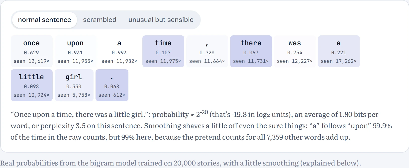
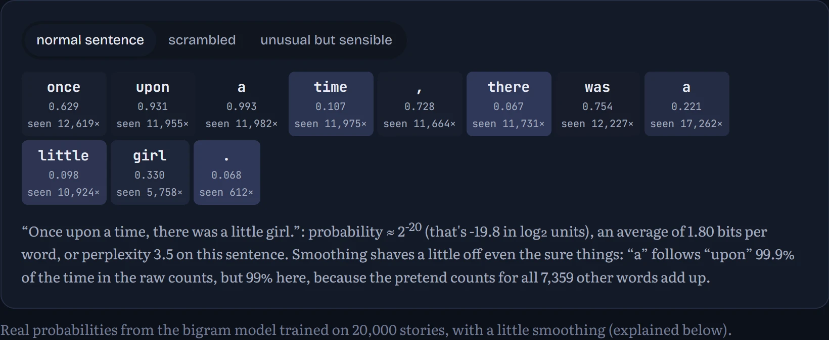
Look at the scrambled sentence: several pairs, like “girl little”, were never seen in training. Pure counting would give them probability exactly 0, and one zero makes the whole sentence's probability 0, however good the rest is. That's too harsh: “purple elephant” appeared just once in 3.8 million words, and plenty of perfectly good pairs never appeared at all. In the held-out stories, 3.2% of word pairs never occurred in training. The fix is smoothing: pretend every possible pair was seen a tiny number of times, k, so nothing is ever impossible. (Chapter 3 shows this is a principled idea, not a hack.)
To compare models with one number, we use perplexity: roughly, how many words the model is choosing between, on average, at each step. A model that guessed uniformly among all 7,359 words in its vocabulary would have perplexity 7,359. Lower is better. How to read the chart: perplexity on 400 stories the models never saw, for three models, on a log scale.
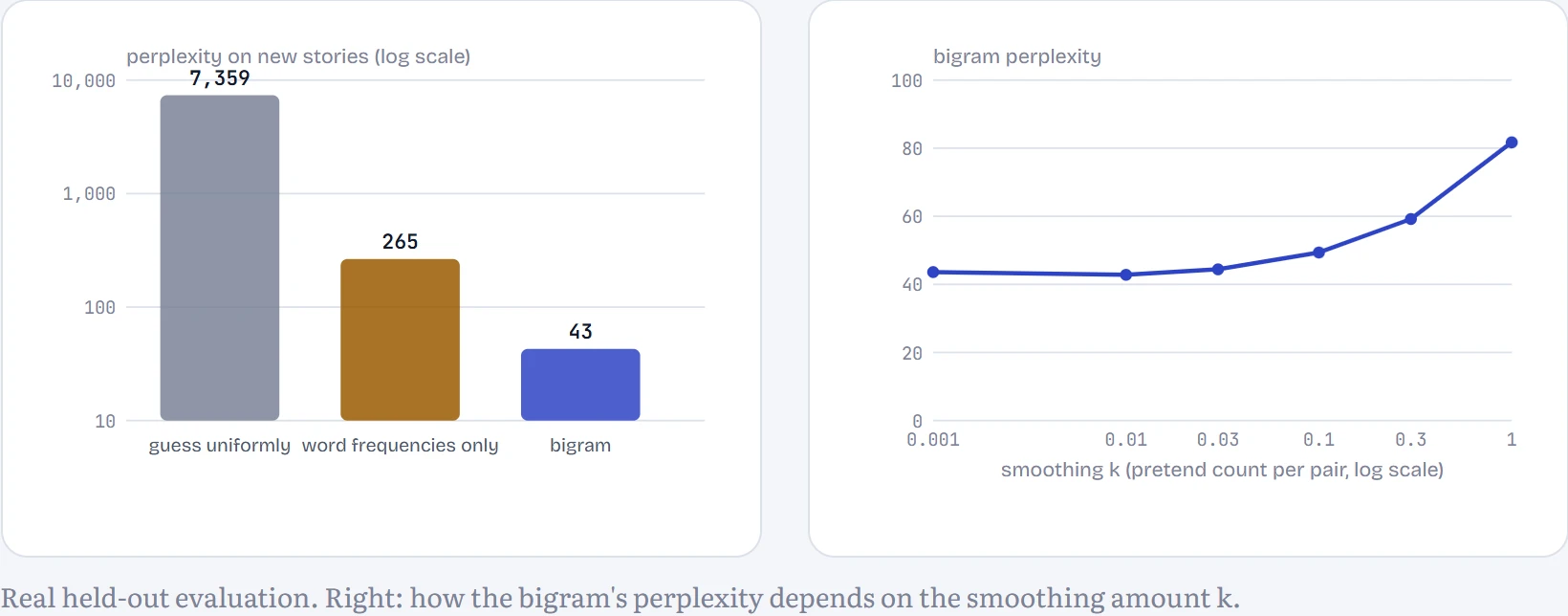
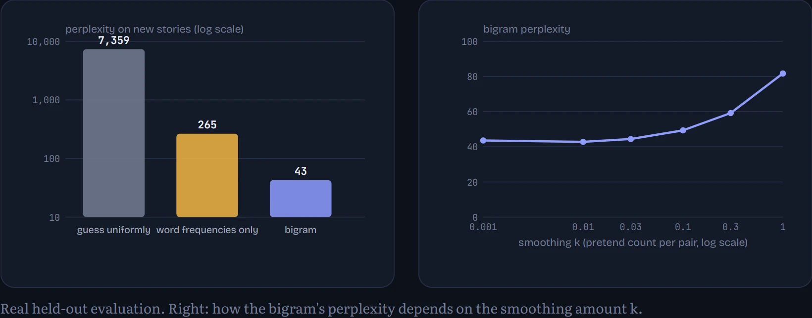
Knowing nothing at all, perplexity would be 7,359. Just knowing how common each word is (“the” is common, “elephant” isn't) brings it down to 265. One word of context brings it to 42.8: on average, the model is as unsure as if it were choosing between about 43 words. The right chart shows why the smoothing amount matters: a tiny pretend count (k = 0.01) is best. Too much smoothing (k = 1) hands so much probability to the thousands of pairs that never happen that the real pairs are starved, and perplexity nearly doubles.
Continue the lesson
The whole lesson, with its drawings and its questions. 7 more sections after the ones above.