
Single-node training: GPU memory accounting, LoRA, ZeRO and FSDP, checkpoint resume and evaluation
Training holds four piles of memory for every model number: weights, gradients, optimizer state and activations. Adam keeps two running averages per weight, created at the first optimizer step, which is why a model that loads can still run out of memory a moment later. Plan the piles before launching.
What this page answers
Why does training fail with CUDA out of memory in adam.py?
Adam keeps its own notes, such as exp_avg, for every number in the model. Those notes did not exist until the optimizer step, and there was no room left for them. Read it in “A 16 GB model that won't fit on an 80 GB GPU”
What uses GPU memory during training?
Weights, often kept at 32-bit precision, 4 bytes each; gradients, another 4 bytes per weight; optimizer state, where Adam keeps two running averages per weight; and the activations of the current step. Read it in “Four piles of memory”
A 16 GB model that won't fit on an 80 GB GPU
You download Llama 3.1 8B. The files on disk add up to 16 GB. You have an H100 with 80 GB of memory, five times the size of the model. You start a full fine-tune (training that changes every number in the model), with just one example of 2,048 tokens (word pieces) at a time. It loads, runs for a few seconds, and dies:
$ python train.py --model meta-llama/Llama-3.1-8B --batch 1 --seq 2048
Loading checkpoint shards: 100%|██████████| 4/4
  File ".../torch/optim/adam.py", in _init_group
    state["exp_avg"] = torch.zeros_like(
torch.OutOfMemoryError: CUDA out of memory. Tried to allocate 224.00 MiB. GPU 0 has a total capacity of 79.19 GiB of which 98.31 MiB is free. Including non-PyTorch memory, this process has 79.09 GiB memory in use. Of the allocated memory 78.42 GiB is allocated by PyTorch, and 142.50 MiB is reserved by PyTorch but unallocated. If reserved but unallocated memory is large try setting PYTORCH_CUDA_ALLOC_CONF=expandable_segments:True to avoid fragmentation.
Error messages, logs and memory figures on this page are realistic examples of PyTorch and Hugging Face output. The commands, settings and formulas are real.
The model is 16 GB and the GPU holds 80 GB. Where did the other 64 GB go?
- The batch of training data
- Training keeps extra numbers for every weight
- PyTorch is leaking memory
Answer. Look at the line just above the error. It died inside adam.py, while the optimizer was making room for something called exp_avg. The optimizer is the part of training that decides how to change each number in the model. Adam, the one almost everyone uses, keeps its own notes about every single number. Those notes didn't exist until this moment, and there was no room left for them.
The model has 8 billion numbers, called parameters or weights. The 16 GB file stores each one in 2 bytes. Training needs about 16 bytes per parameter, before counting any training data at all. 8 billion times 16 bytes is 128 GB. That will never fit on one 80 GB GPU, however small you make the batch. The next section shows what those 16 bytes are.
What training actually does
Before counting memory, it helps to see what training is doing with it. Training is a loop of four steps, repeated millions of times. Forward: the model makes a prediction for a batch of examples, using its current weights. Loss: one number measures how wrong those predictions were. Backward: for every weight, work out which direction to nudge it, and how strongly, to make the loss smaller. That direction is the weight's gradient. Step: the optimizer nudges every weight a little along its gradient. Then the next batch, and again.
In PyTorch, the whole loop is a handful of lines. Everything else in a training script, and most of this lesson, is about making these lines fit in memory and survive for days:
for batch in loader:                      # one pass over all batches is an epoch
    out  = model(batch["input_ids"])         # forward: predict
    loss = loss_fn(out, batch["labels"])     # one number: how wrong
    loss.backward()                          # backward: a gradient for every weight
    optimizer.step()                         # nudge the weights
    optimizer.zero_grad()                    # clear the gradients for the next batch
Here's that loop running for real, on the smallest possible model: two weights, a slope and a starting height, learning to draw a line through 20 points. The learning rate decides how big each nudge is. The other learning rates:
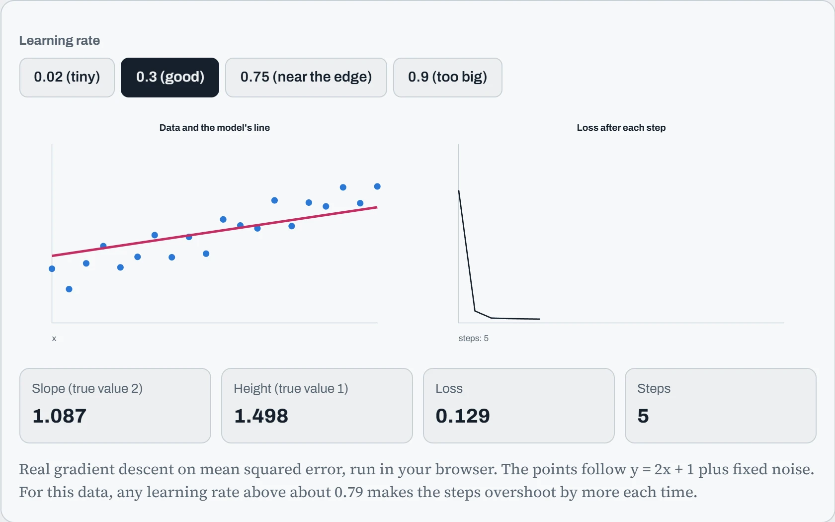
At 0.3 the line settles in a few dozen steps. At 0.02 it's heading the right way but would take many hundreds of steps. At 0.75 it zig-zags but still settles, and at 0.9 every step overshoots further than the last until the numbers explode. Big models behave the same way with billions of weights instead of two: too high a learning rate, and the loss jumps to nan; too low, and you pay for GPU hours that barely move it. That's why learning rates for fine-tuning are tiny numbers like 0.0002, and why every run is watched through its loss curve.
The same loop covers every kind of training you'll meet in this course. They differ only in where the examples and the loss come from:
| Kind | Examples | The loss says | Scale |
|---|---|---|---|
| Pretraining | Trillions of tokens of ordinary text | How badly did you guess each next token? | Thousands of GPUs, months |
| Fine-tuning (SFT) | Thousands of example conversations | How far was your answer from the example answer? | One machine, hours |
| Reinforcement learning | Questions, and a way to score answers | Do more of what scored well, less of what scored badly | One machine to a cluster |
This chapter is about the middle row, on one machine, plus the last row at the end. The rest of the lesson is about the cost of that innocent-looking loss.backward() and optimizer.step(): both need extra numbers for every weight, and that's where the memory goes.
Four piles of memory
Think of training like a student correcting a long essay. To do it properly they need four things on the desk at once. Training needs the same four, for every one of the model's numbers.
The weights are the essay itself: the model's numbers. During training they're usually kept in full 32-bit precision, 4 bytes each, so that tiny corrections don't get rounded away.
The gradients are the red-pen notes: for each weight, which direction to nudge it and by how much. One note per weight, another 4 bytes each.
The optimizer state is the student's memory of past corrections. Adam keeps two running averages for every weight: one of the recent nudges, and one of how big the nudges have been. That's 4 bytes each, so 8 bytes per weight. This is the exp_avg from the error.
The activations are scratch work. As data flows forward through the model, each layer's in-between results get saved, because the backward pass (the step that works out the gradients) needs them. Unlike the other three, this pile depends on how much data you push through at once, not just on the model.
Add the first three and you get 4 + 4 + 8 = 16 bytes for every weight. Some setups split it differently, for example a 2-byte working copy plus a 4-byte master copy, but it still comes to about 16. The picture below draws all of it to scale for the 8B model, next to the file you downloaded. The dashed pink line is the 80 GB GPU. Everything to its right doesn't fit.
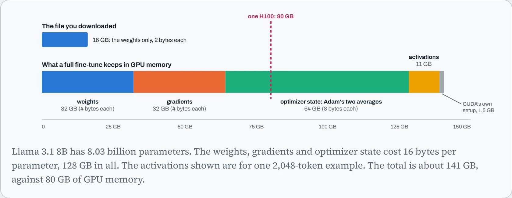
Two things stand out. The file on disk is only a small piece of what training needs, about one eighth. And Adam's notes alone take 64 GB, four times the size of the model you downloaded. When people say a model “needs an 80 GB GPU”, they usually mean running it. Training it is a different budget.
Predict. You double the batch, from one example at a time to two. Which of the four piles get bigger?
Answer. Only the activations. The weights, gradients and Adam's notes depend on how many numbers the model has, not on how much data you feed it. So the first three piles stay exactly the same, and only the scratch work doubles, from about 11 GB to about 22 GB.
This gives you two kinds of fixes. Changing the batch or the sequence length only touches the activations. To shrink the other three piles, you have to change how you train. That's the next section.
Shrinking the piles
The biggest saving comes from a simple idea: don't change all 8 billion numbers. For most fine-tuning jobs, like teaching a model a format, a tone or a narrow skill, you only need to nudge it a little. LoRA (low-rank adaptation) freezes the original weights and trains a small add-on next to each layer instead.
Here's how the add-on works. Inside the model, a layer multiplies its input by a big grid of numbers. In Llama 3.1 8B, some of these grids are 4,096 by 4,096, about 16.8 million numbers each. LoRA leaves that grid alone and adds two thin grids next to it. One is 4,096 by 16 and the other is 16 by 4,096. Multiplied together, they make a full-size correction to the big grid, but they only have 131,072 numbers between them. The 16 is called the rank, and you choose it. In the picture, blue means “trained” and grey means “frozen”.
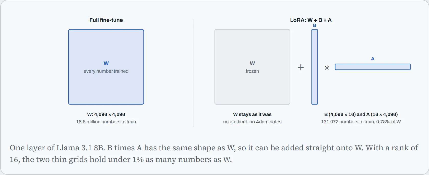
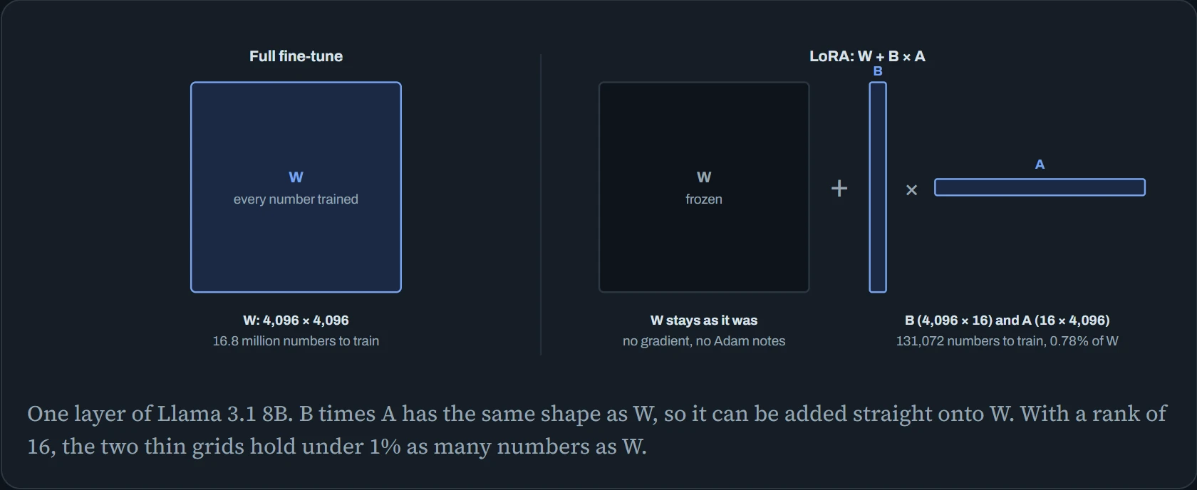
The frozen weights still sit in GPU memory, because data has to flow through them. But they need no gradients and no Adam notes. All 16 bytes per parameter are now spent only on the small add-on. PEFT, the Hugging Face library for this, tells you how small it is:
>>> from peft import LoraConfig, get_peft_model
>>> cfg = LoraConfig(r=16, lora_alpha=32, target_modules="all-linear", task_type="CAUSAL_LM")
>>> model = get_peft_model(model, cfg)
>>> model.print_trainable_parameters()
trainable params: 41,943,040 || all params: 8,072,204,288 || trainable%: 0.5196
About 42 million numbers to train instead of 8 billion. The gradients and Adam's notes drop from 96 GB to about half a gigabyte. The frozen weights, kept at 2 bytes each, are now the biggest pile at 16 GB.
QLoRA goes one step further and shrinks that pile too. It stores the frozen weights in 4 bits (half a byte) each, in a format called NF4, and unpacks them on the fly as each layer runs. The 8B model's frozen weights drop to under 6 GB. Not every layer gets packed this way: the tables that turn words into numbers and back stay at 2 bytes, which is why it's nearly 6 GB and not 4. The trainable add-on stays at full precision, so the learning itself isn't done in 4 bits.
>>> bnb = BitsAndBytesConfig(load_in_4bit=True, bnb_4bit_quant_type="nf4",
...                          bnb_4bit_use_double_quant=True, bnb_4bit_compute_dtype=torch.bfloat16)
>>> model = AutoModelForCausalLM.from_pretrained("meta-llama/Llama-3.1-8B", quantization_config=bnb)
>>> model.get_memory_footprint() / 1e9
5.59
LoRA and QLoRA shrink the first three piles. The activations need different fixes, and so does the case where you really do need to change every weight. Here's the full set of levers, with what each one costs you.
| Change | What it does | Pile it shrinks | What it costs |
|---|---|---|---|
| LoRA | Freezes the model and trains a small add-on | Gradients and optimizer state, almost to nothing | Can't change the model as deeply as a full fine-tune |
| QLoRA | LoRA, plus the frozen weights stored in 4 bits | The weights too, to between a quarter and a third | Slower steps (unpacking 4-bit numbers), and slightly lower quality |
| Gradient checkpointing | Saves only each layer's input. During the backward pass it redoes the forward work for one layer at a time | Activations, often by 5 to 10 times | Steps take roughly 20 to 30% longer, because some work is done twice |
| Smaller micro-batch plus gradient accumulation | Runs fewer examples at once and adds up the gradients over several runs before updating | Activations | More, smaller steps. The training result is about the same |
| 8-bit Adam | Stores Adam's two averages in 1 byte each instead of 4 | Optimizer state, from 8 bytes per weight to 2 | Needs the bitsandbytes library. A small risk of less stable training |
| FSDP across N GPUs | Fully Sharded Data Parallel: each GPU keeps 1/N of the weights, gradients and Adam notes, and they swap pieces as needed | The first three piles, divided by N | Needs more GPUs, plus a lot of traffic between them (Down the Wire) |
Notice that nothing on this list is free. Each one trades memory for something else: time, quality, or more hardware. The skill is picking the cheapest trade for your job. That's easier to feel than to read, so the next section lets you try them.
Plan before you launch
Finding out about memory by crashing is slow, and on a rented GPU it's expensive. The planner below does the sums from the last two sections, so you can check a setup before you start it.
How to read it: the bar is everything one GPU must hold, split into the four piles plus a small slice for CUDA itself. The dashed pink line is your GPU's memory. If the bar ends left of the line, it fits. The number after each pile tells you where to look first. These are estimates. A real run needs some slack on top, for reasons the allocator section explains.
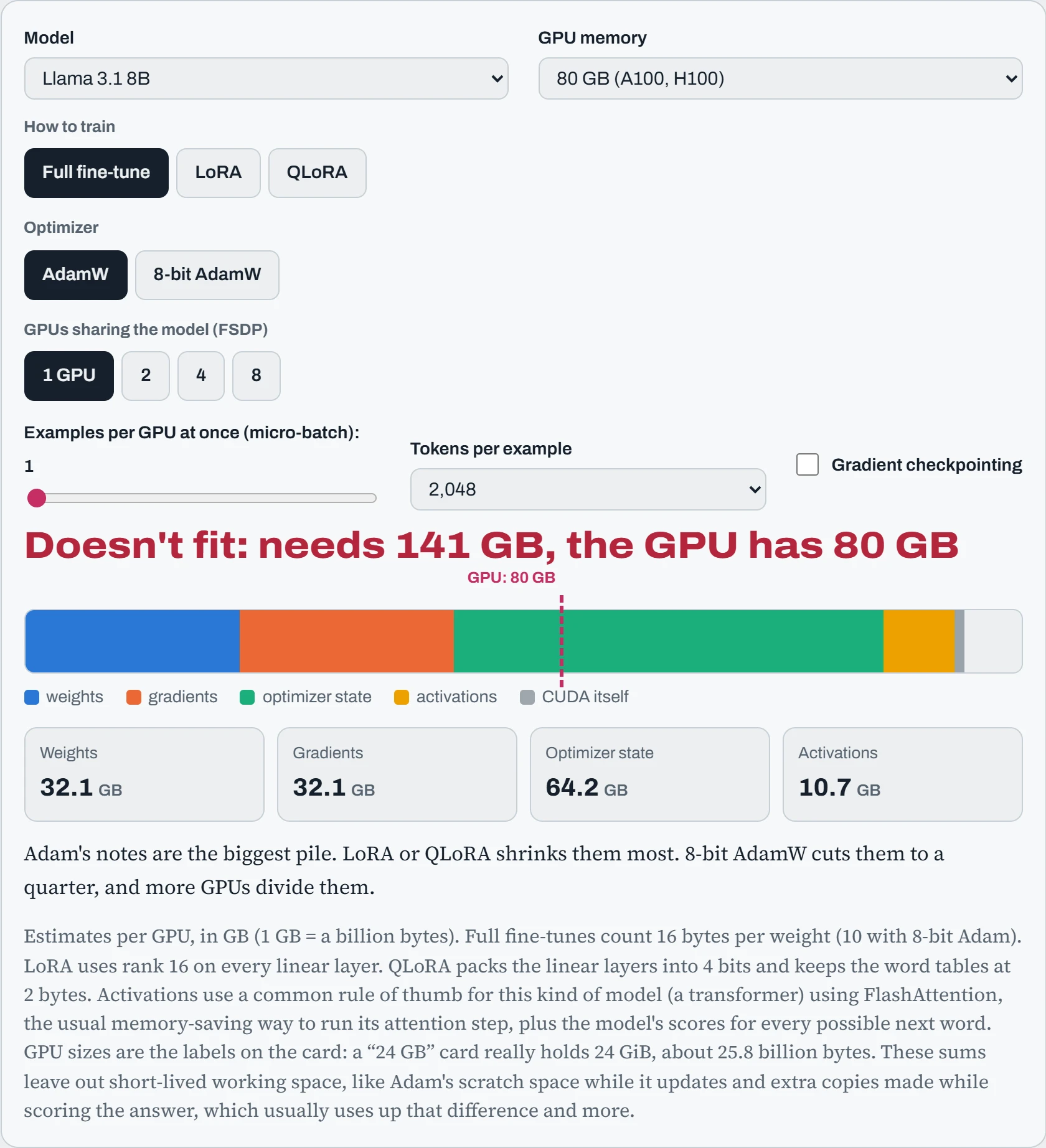
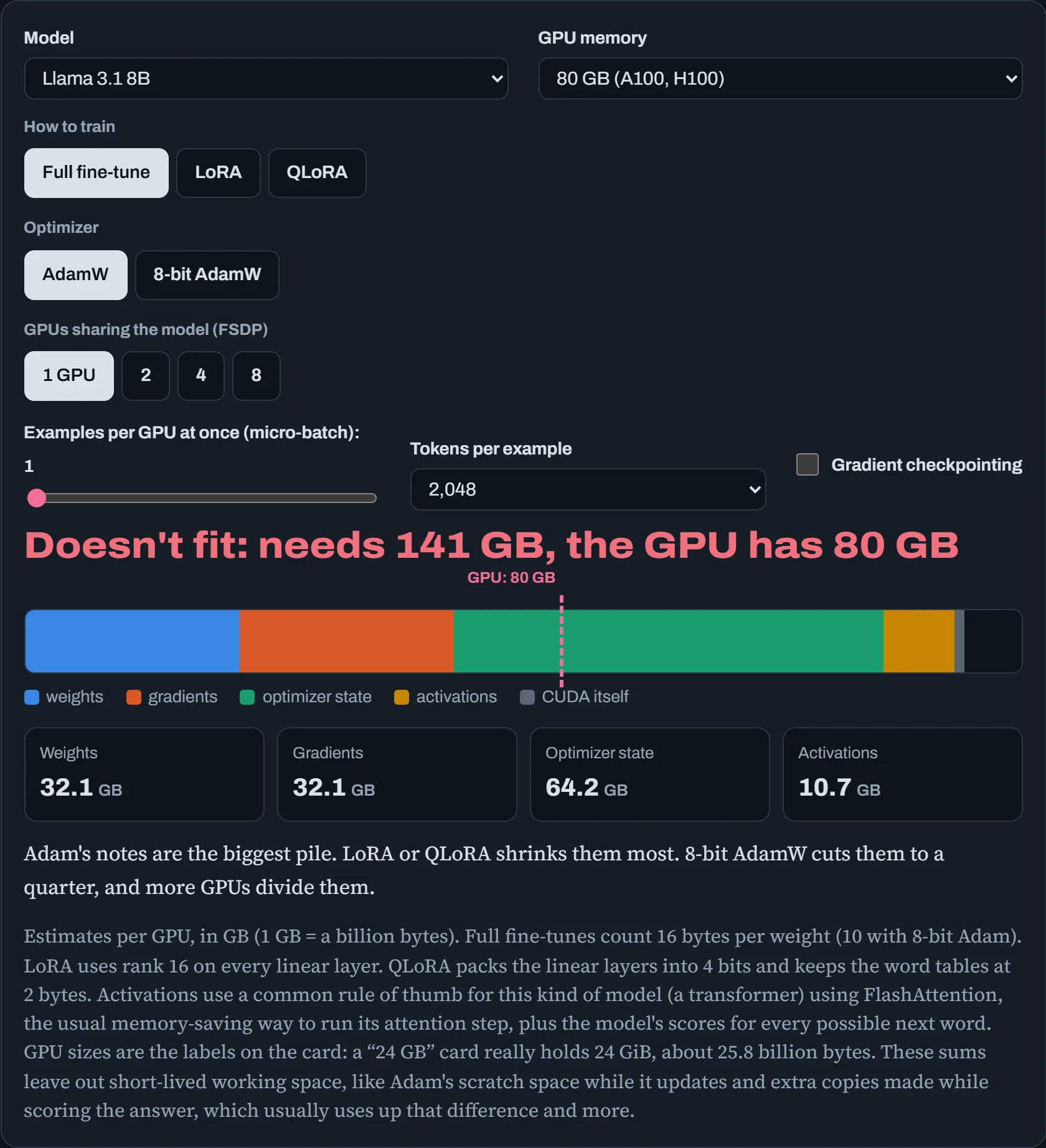
The default first: a full fine-tune of the 8B model on one 80 GB GPU. It needs about 141 GB, as the four-piles picture showed. Now switch to 8 GPUs. The first three piles split eight ways, to 16 GB per GPU in all, and it fits. On 1 GPU with LoRA, it fits on one card. With QLoRA and checkpointing on, it even fits on a 24 GB gaming card.
One pile doesn't follow the pattern. At 8,192 tokens per example, the amber activations grow. Gradient checkpointing tames most of them, but a stubborn chunk is left over. That's the model's score for every possible next word, about 128,000 of them, kept for every token. On long sequences that alone can be several gigabytes.
Predict. You have one 80 GB GPU and want to fine-tune Llama 3.1 70B. What's the cheapest setup that fits? Make a guess, then check it in the planner.
Answer. QLoRA with gradient checkpointing, one example of 2,048 tokens at a time: about 49 GB. Plain LoRA doesn't fit, because the frozen weights alone are 141 GB at 2 bytes each. Even a full fine-tune spread over 8 GPUs doesn't fit, since 16 bytes times 70.6 billion, divided by 8, is still 141 GB per GPU.
This is why QLoRA made such a splash. Before it, tuning a 70B model needed several big GPUs. With it, one card is enough. It's not free: steps are slower, because the 4-bit weights have to be unpacked again and again.
Surviving a restart
A fine-tune that fits in memory can still die. A cloud provider takes back your cheap “spot” machine, a scheduler stops your job to make room for someone else's, the power blips, or you close the laptop that held your SSH session. A run that can't restart where it left off loses everything since it began.
Making a run restartable takes three habits. Save often: write a checkpoint (a saved copy of the run's state) every few hundred steps. Save everything: the model alone isn't enough. To carry on exactly where you were, you also need Adam's notes, the learning-rate schedule's position (the plan for how big each nudge may be, which changes as training goes on), the step number, and the random number generators' state. Save safely: write to a temporary file first, then rename it. A rename happens all at once, so a crash halfway through a save can never leave you with a broken checkpoint.
Here's a loop that does all three. It also listens for SIGTERM, the polite “please stop” signal that Linux sends before it forces a program to quit (chapter 5).
import os, signal, torch

stop = False
def on_sigterm(signum, frame):
    global stop
    stop = True                       # just set a flag; save at a safe point
signal.signal(signal.SIGTERM, on_sigterm)

def save(path, step):
    tmp = path + ".tmp"
    torch.save({"model": model.state_dict(), "optim": opt.state_dict(),
                "sched": sched.state_dict(), "step": step,
                "cpu_rng": torch.get_rng_state(),
                "cuda_rng": torch.cuda.get_rng_state()}, tmp)
    os.replace(tmp, path)             # atomic rename: never a half-written file

start = 0
if os.path.exists("ckpt/last.pt"):
    state = torch.load("ckpt/last.pt", map_location="cpu")
    model.load_state_dict(state["model"]); opt.load_state_dict(state["optim"])
    sched.load_state_dict(state["sched"])
    torch.set_rng_state(state["cpu_rng"]); torch.cuda.set_rng_state(state["cuda_rng"])
    start = state["step"] + 1

for step in range(start, total_steps):
    train_one_step(step)
    if step % 500 == 0 or stop:
        save("ckpt/last.pt", step)
    if stop:
        break
Two details matter here. The signal handler only sets a flag. It never saves from inside the handler, because the signal can arrive halfway through a step, when the weights are partly updated. And the data has to resume too. Either skip the batches you've already used, or use a data loader that can save its own position, like torchdata's StatefulDataLoader. If you use the Hugging Face Trainer, it does the saving and resuming for you, including skipping the data it already used: trainer.train(resume_from_checkpoint=True) picks up the latest checkpoint in the output folder. It doesn't listen for SIGTERM, though, so its regular saves are what protect you.
Now the catch. After SIGTERM, you only get a short grace period. Then comes SIGKILL, which can't be caught, and the program is gone. Whether a last-moment save finishes in time depends on three things: how big the checkpoint is, how fast the disk is, and how long the grace period is. The copper bar is the time the save takes. The pink line is when the kill arrives.
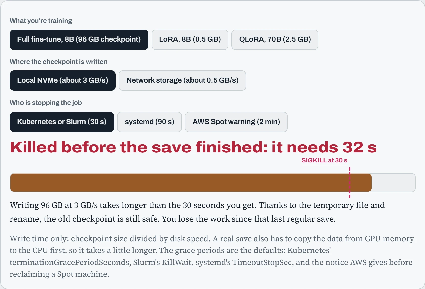
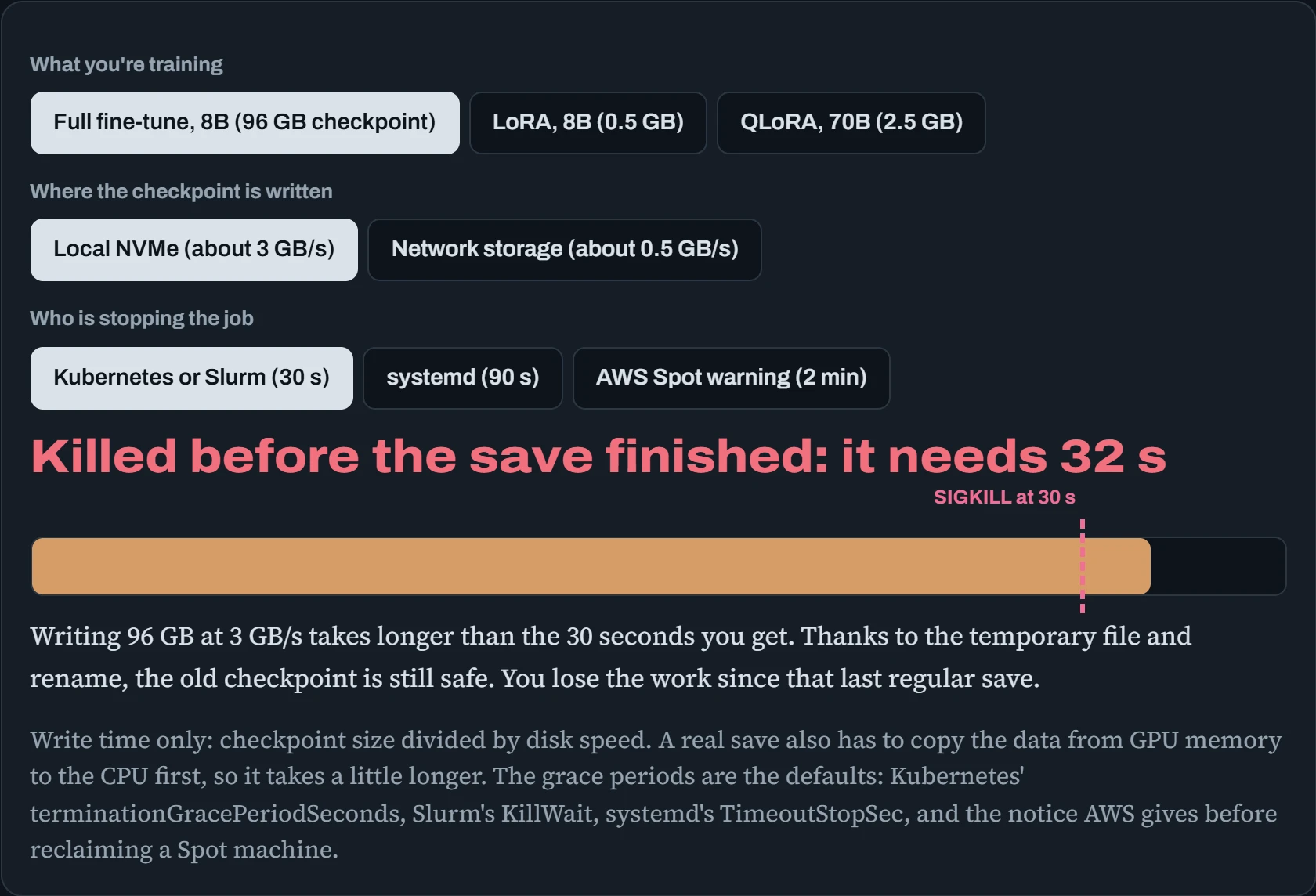
The full fine-tune is the trap. Its checkpoint is 96 GB: the 32 GB of weights plus 64 GB of Adam's notes (gradients aren't saved, because they're recomputed every step). Even on a fast local disk, that takes about 32 seconds, just over Kubernetes' 30. So never count on the last-second save. Treat it as a bonus, and rely on regular checkpoints. Then the most a kill can cost you is the work since the last one.
Big checkpoints cause a second problem: they fill disks. Ten 96 GB checkpoints is nearly a terabyte. Keep only the last two or three (the Trainer's save_total_limit=2 does this), and put checkpoints on their own disk or partition, so a full checkpoint disk can't also take down the operating system or your data.
Finally, the job should restart by itself. In a terminal, tmux keeps it alive when your SSH connection drops. But a systemd service (chapter 10) also restarts it after a crash, logs to a file, and controls the grace period:
# /etc/systemd/system/finetune.service
[Unit]
Description=Fine-tune job

[Service]
User=train
WorkingDirectory=/srv/train
Environment=PYTHONUNBUFFERED=1    # write output to the log right away
Environment=PYTORCH_CUDA_ALLOC_CONF=expandable_segments:True
Environment=TORCHINDUCTOR_CACHE_DIR=/srv/cache/inductor
ExecStart=/srv/train/.venv/bin/python train.py
Restart=on-failure                # crashed? start again; the loop resumes from ckpt/last.pt
RestartSec=60
TimeoutStopSec=120                # "stop" sends SIGTERM, waits 120 s, then SIGKILL
StandardOutput=append:/srv/train/logs/train.log
StandardError=append:/srv/train/logs/train.log

[Install]
WantedBy=multi-user.target        # start at boot after: systemctl enable finetune
The first Environment line stops Python from holding its output back, so the log is always up to date. The other two will make sense soon. One tells PyTorch to handle memory in a way that avoids gaps, and the other keeps compiled GPU code somewhere that survives a restart. Both come up again in the symptoms section.
Picking a fine-tuning toolchain
You rarely write a training loop from scratch. A handful of toolchains do the work, and they differ mainly in how you drive them: by writing Python, by editing a config file, or by clicking in a web page. Underneath, most use the same pieces: Hugging Face Transformers for the model, PEFT for LoRA adapters, and TRL for training recipes like supervised fine-tuning (SFT).
| Toolchain | How you drive it | Good at |
|---|---|---|
| TRL + PEFT | Python code, or the trl command | Full control, every method, the reference others build on |
| Unsloth | Python code | Fast, memory-lean LoRA and QLoRA on a single GPU |
| Axolotl | One YAML config file | Repeatable runs, multi-GPU and multi-node, many dataset formats |
| LLaMA-Factory | Config file, or a web UI | Trying many models and methods quickly |
| torchtune | Config file and ready-made recipes | Pure PyTorch, few extra dependencies |
Which one to start with depends on your hardware and how you like to work.
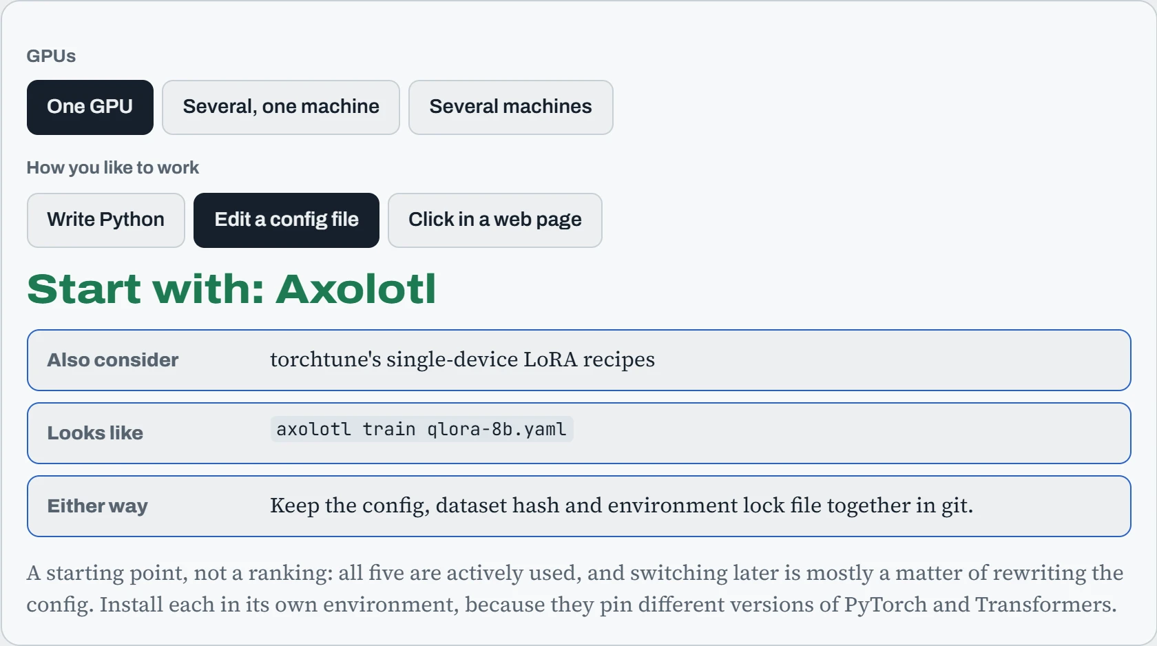
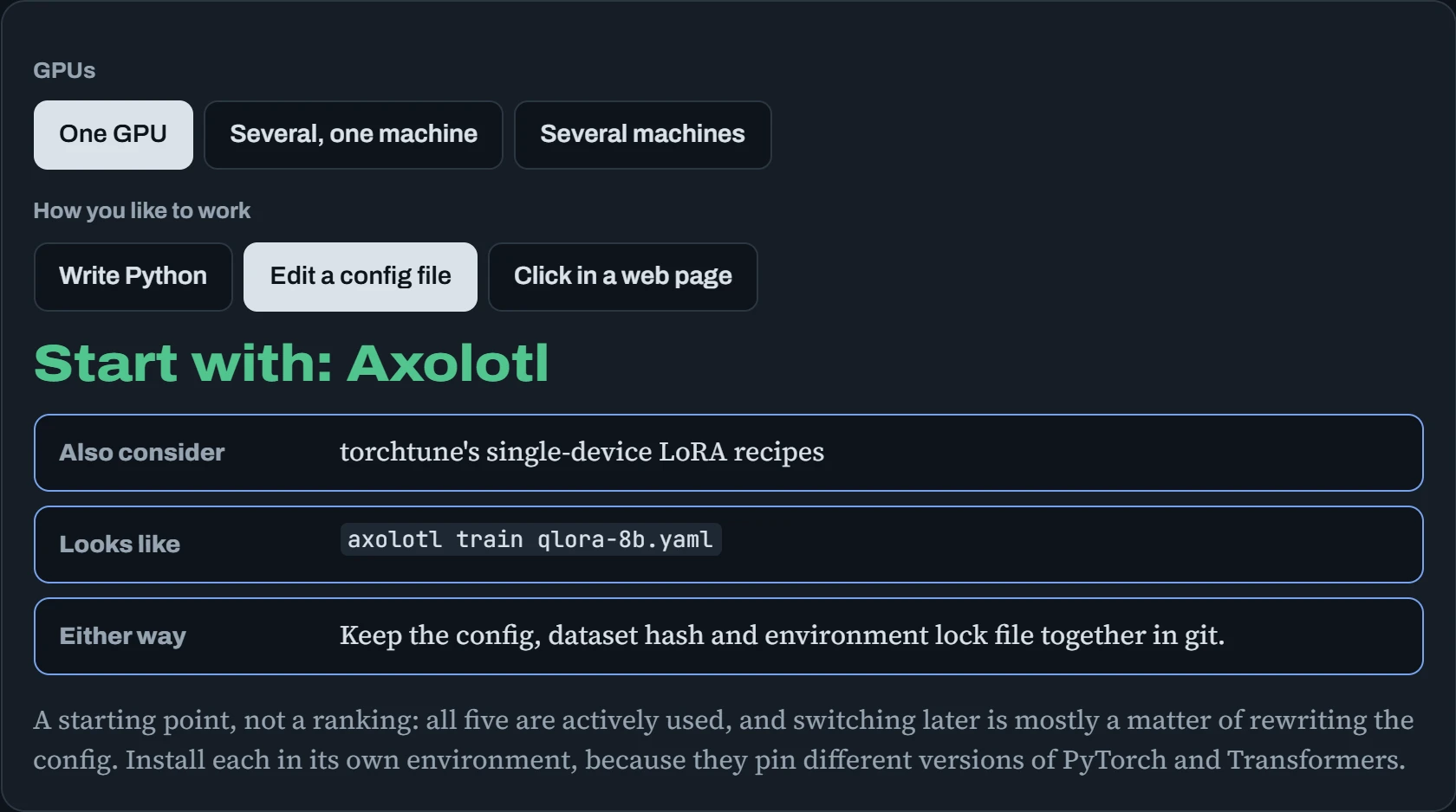
Whichever you pick, the run should be described by files you can commit: a config, a dataset hash, a pinned environment (Down the Path). Here's what that looks like with Axolotl, where the whole QLoRA run from the lab is one file:
# qlora-8b.yaml
base_model: meta-llama/Llama-3.1-8B-Instruct
load_in_4bit: true
adapter: qlora
lora_r: 16
lora_alpha: 32
datasets:
  - path: data/train.jsonl
    type: chat_template
sequence_len: 4096
micro_batch_size: 2
gradient_accumulation_steps: 8
num_epochs: 3
learning_rate: 0.0002
gradient_checkpointing: true
output_dir: runs/qlora-8b
$ axolotl train qlora-8b.yaml
Every setting from the planner above appears here by name: 4-bit loading, LoRA rank, batch size, gradient checkpointing. That's the real advantage of config-driven tools: the file is the record of what you ran.
Continue the lesson
The whole lesson, with its drawings and its questions. 8 more sections after the ones above.